Download
1 / 1
10 likes | 147 Views
Quantitative network design for biosphere model process parameters E. Koffi 1 , P. Rayner 1 , T. Kaminski 2 , M. Scholze 3 , M. Voßbeck 2 , and R. Giering 2 1 Laboratoire des Sciences du Climat et de l’Environnement (LSCE), Gif-sur-Yvette, France (ernest.koffi@lsce.ipsl.fr)

E N D
Quantitative network design for biosphere model process parameters E. Koffi1, P. Rayner1, T. Kaminski2, M. Scholze3, M. Voßbeck2, and R. Giering2 1Laboratoire des Sciences du Climat et de l’Environnement (LSCE), Gif-sur-Yvette, France (ernest.koffi@lsce.ipsl.fr) 2FastOpt , Hamburg, Germany 3Quantifying and Understanding the Earth System, Department of Earth Sciences, University of Bristol, United Kingdom Figure 3: The CO2 network consists of 41 Global View (GV) flask sites (+), 2 continuous measurement sites (x) and an Eddy flux measurement site ( ). Green color stands for the sites used for the network evaluation. Redcolor stands for sites that are not used. Two candidate networksare evaluated: Network 1 consists of 41 GV stations Network 2 consists of 37 GV stations, excluding 4 sites over Europe ( ) For further details on the Network Design Tool, contact Thomas kaminski (Thomas.Kaminski@FastOpt.com) or consult http://imecc.ccdas.org Set up • The network designer allows to handle (Figure 2): • Flask sampling of atmospheric CO2, using the transport model TM2 as observational operator. • Continuous samples for atmospheric CO2, using the atmospheric transport model LMDZ as observational operator. • Direct flux observations. Figure 2: Carbon Cycle Assimilation System (CCDAS). Forward modelling chain together with the modules for full network design tool. This work was supported in part by the European Commission under contract numbers FP6-511176-2 (CarboOcean) and FP6-026188 (IMECC) Background and Motivation Current uncertainty about the present and future behaviour of the terrestrial carbon cycle has stimulated the research community to build appropriate observing networks. Quantitative network design, based on inverse modelling systems aims to optimize such networks. This approach is used, in the framework of the European project IMECC (Infrastructure for Measurement of the European Carbon Cycle), to evaluate candidates of networks that better constrain the process parameters of a biospheric model. The impact of various atmospheric and terrestrial measurements on the uncertainty of process parameters and concomitant uncertainty of calculated fluxes is demonstrated, along with a tool for assessing networks. Methodology Carbon Cycle Data Assimilation System The network design tool is based on the CCDAS (Carbon Cycle Data Assimilation System) (Figure 1). The system consists of the terrestrial biosphere model BETHY (Biosphere Energy Transfer Hydrology) (Knorr, 2000), which can couple with several atmospheric transport models (e.g., Scholze, 2003, Rayner et al., 2005). CCDAS allows the calculation of diagnostic (Rayner at al., 2005) and prognostic (Scholze et al., 2007) quantities. Network Design Tool and First Applications Application to CO2 fluxes The tool has been used to evaluate candidate networks for the carbon cycle study, using only flask samples of atmospheric CO2 as observations. We focused on the CO2 fluxes. The uncertainty on the CO2 data [σdi] that reflects the combined effect of observational and model error was set to 2 ppmv for each flask. The Uncertainties on the Net Ecosystem Production NEP (net CO2 flux between the atmosphere and the biosphere) and the Net Primary Production NPP of the biosphere are calculated for the two networks ofFigure 3. Table 1: Uncertainties on NPP and NEP evaluated from Network 1(41 stations, green) and Network 2(37 stations, blue). The prior uncertainties of these quantities are also reported (black). Uncertainties on NPP and NEP decrease by more than 87% and 89% respectively, when using all the GV sites (Table 1). For the case under study, the exclusion of 4 stations does not significantly alters this reduction (i.e. less than 1%). • Figure 1: The two-steps procedure for inferring diagnostic and prognostic target quantities from CCDAS. • Rectangular boxes: processes. • Oval boxes: data • Diagonally hatched box: inversion or calibration step. • Vertical hatched box: diagnostic step. • Horizonally hatched box: prognostic step. Formalism of the network design tool Themethod is based on the assessment of candidate networks of carbon cycle measurements through the computation of the uncertainty on a target quantity (Kaminski and Rayner, 2008). The method solves an inverse problem, which is formulated as a minimization of a cost function J(x): (1) Uncertainty on a target quantity If the model M is linear, the data d and the priors of the parameters x have a Gaussian Probability Density Function (PDF), then the posterior (i.e., optimized) values of x also have a Gaussian PDF (Tarantola, 1987). The posterior uncertainty C(xop) is given by the inverse of the Hessian H (i.e., the second derivative) of the cost function J(x) (equation 1). Following Rayner et al., 2005, the uncertainty C(y) of a target quantity y(x) is approximated to first order by the equation (2). References Kaminski T. and P. J. Rayner (2008), Assimilation and network design. In H. Dolman, A. Freibauer, and R. Valentini, editors, to appear in Observing the continental scale Greenhouse Gas Balance of Europe, Ecological Studies, chapter 3. Springer-Verlag, New York Knorr W. (2000), Annual and interannual CO2 exchanges of the terrestrial biosphere: process based simulations and uncertainties, Glob. Ecol. And Biogeogr., 9:225-252 Tarantola, A. (1987), Inverse problem theory – Methods for data fitting and model parameter estimation. Elsevier Science, New York, USA, 1987 Rayner, P.J., M. Scholze, W. Knorr, T. Kaminski, R. Giering, and H. Widmann (2005), Two decades of terrestrial carbon fluxes from a carbon cycle data assimilation system (CCDAS), Global Biogechen. Cycles, 19, GB2026, Doi:10..1029/2004GB002254 Scholze, M, (2003), Model studies on the response of the terrestrial carbon cycle on climate change and variability, Examensarbeit, Max-Planck-Inst. Für Meterol., Hamburg, Germany Scholze, M., T. Kaminski, P. Rayner, W. Knorr, and R. Giering (2007), Propagating uncertainty through prognostic carbon cycle data assimilation system simulations. J. Geophys. Res., 112, D17305, doi:10.1029/2007JD008642 (2)