Download
1 / 62
620 likes | 778 Views
Generic, Deformable Models for 3-D Vehicle Surveillance. Matthew Leotta Ph.D Thesis Defense September 2, 2009. Motivating Example 1: 3-D Traffic Monitoring. 3-d road models are used in traffic reports Raw traffic video shows what is really happening

E N D
Generic, Deformable Models for 3-D Vehicle Surveillance • Matthew Leotta • Ph.D Thesis Defense • September 2, 2009
Motivating Example 1:3-D Traffic Monitoring • 3-d road models are used in traffic reports • Raw traffic video shows what is really happening • Can the actual traffic images be mapped into a 3-d traffic model? [Triangle Software]
Motivating Example 2:3-D Facility Monitoring • Monitor vehicle traffic for security on a campus or base • Want to recognize vehicles and track them from camera to camera • Can this be automated and integrated into a single world map?
3-D Surveillance Objectives • Primary thesis objective: • Dense 3-d shape recovery of vehicles from 2-d images • Secondary thesis objectives: • Vehicle tracking in 3-d (jointly with shape estimation) • Vehicle class recognition (from recovered shape) four-door sedan
Overview • The approach: A 3-d deformable model • Learning the shape deformations • Fitting the model to images (shape and pose) • Tracking the model in video • Vehicle class recognition in shape space
Overview • The approach: A 3-d deformable model • Learning the shape deformations • Fitting the model to images (shape and pose) • Tracking the model in video • Vehicle class recognition in shape space
Previous Work:Deformable 3-D Vehicles • Deformable 3-d model fits many vehicle classes • Model edges are matched to lines, which are fit from detected edges Ferryman et al. BVMC 1995 Koller et al. IJCV 1993 [Kolleret al. IJCV 1993, Ferryman et al. BMVC 1995]
Previous Work:Complex 3-D Vehicle Meshes • Use highly complex vehicle meshes (~100K faces) from CAD • Predict vehicle high resolution appearance over viewpoint change Guo et al. CVPR 2008 [Guoet. al. CVPR 2008]
E3D CAD Models • 79 Passenger Vehicles from DARPA’s Exploitation of 3-D Data (E3D) project • Six vehicle classes • SUV • Minivan • Pickup truck • Two-door sedan • Four-door sedan • Station wagon
Detailed, Deformable Vehicle • The proposed model • Requirements • Adaptive mesh complexity • Deformable 3-d mesh • Deformable 2-d vehicle parts • Small number of shape parameters
Subdivision Surface Vehicle generic, but too simple too specific, too complex • Subdivision adapts the complexity of the mesh as needed generic with adaptable complexity
Texture Mapped Parts • Texture space is a mapping of the mesh vertices to the unit square • Parts are polygons in 2-d texture space • Part boundaries are not restricted to mesh edges Texture Space
Overview • The approach: A 3-d deformable model • Learning the shape deformations • Fitting the model to images (shape and pose) • Tracking the model in video • Vehicle class recognition in shape space
Mesh Model Learning • Shrink-wrap mesh to implicit surface of polygon soup[Shenet al. SIGGRAPH 2004] • Recursively fit the subdivided mesh body
Mesh Model Learning • Shrink-wrap mesh to implicit surface of polygon soup[Shenet al. SIGGRAPH 2004] • Recursively fit the subdivided mesh body
Mesh Model Learning • Shrink-wrap mesh to implicit surface of polygon soup[Shenet al. SIGGRAPH 2004] • Recursively fit the subdivided mesh body
Mesh Model Learning • Shrink-wrap mesh to implicit surface of polygon soup[Shenet al. SIGGRAPH 2004] • Recursively fit the subdivided mesh body
Training Part Extraction • Map CAD model parts to the closest point on the deformable mesh • Map boundaries into texture space
Part Model Learning • Apply the analogous 2-d shrink wrap to the parts • Implicit surface is not needed • Convex hull used for initial fit
Part Model Learning • Apply the analogous 2-d shrink wrap to the parts • Implicit surface is not needed • Convex hull used for initial fit
Principal Components • PCA reduces the space of shape parameters • The top 5 principal component of the vehicle model deviation 1 2 3 4 5
Overview • The approach: A 3-d deformable model • Learning the shape deformations • Fitting the model to images (shape and pose) • Tracking the model in video • Vehicle class recognition in shape space
Edge Prediction • Predict the most salient intensity edges with • Occluding contours • Part boundaries
Jacobian Error Vector Parameter Update Optimizing Parameters • Shape and pose • Gauss-Newton minimization • Iterative least-squares to minimize edge distances
Identity Matrix Negative of Current Parameters Regularization • Use Tikhonov regularization • A Gaussian prior in Bayesian terms
Scaled Inverse Standard Deviations Regularization (Normalized) • controls the amount of regularization • normalizes the shape parameters • zeroed for pose parameters
Diagonal Weight Matrix Robust Estimation • Iteratively reweighted least-squares • Beaton-Tukey M-estimator • Other heuristic weights
Multi-Scale Optimization Scale = 8 Scale = 4 • Plot show magnitude of the residual: • Start with coarse scale and progress to fine scale. Scale = 2 Scale = 1
Poor Initialization High Initial Uncertainty Good Initialization Low Initial Uncertainty Ferryman Dodecahedral Detailed 2 Detailed 1 Detailed 3 Number of PCA Parameters • 5 shape parameters balance expressiveness with over fitting
Chevrolet S10 Blazer Dodge Caravan Dodge Stratus Nissan Maxima Toyota 4Runner Toyota Tundra VW Beetle (black) VW Beetle (yellow) Volvo V70XC Multi-view Fitting
Chevrolet S10 Blazer Dodge Caravan Dodge Stratus Nissan Maxima Toyota 4Runner Toyota Tundra VW Beetle (black) VW Beetle (yellow) Volvo V70XC Multi-view Fitting
- RMS Error (meters) - RMS Error (meters) Z Angle (degrees) Z Angle (degrees) X Distance (meters) X Distance (meters) Pose Convergence Regions Dodge Stratus • Initial pose sampled on a regular grid in a 2-d subspace • X distance • Z angle • A plateau indicates a region of stable convergence • Toyota 4Runner has a dual plateau Z X Toyota 4Runner
Convergence Results • Mean Initial Shape • Random Initial Pose • Uniform in angle mag. • Uniform in distance • Uniform directions on the sphere • 10 samples per bin Number Converged Distance (meters) Angle (degrees)
Overview • The approach: A 3-d deformable model • Learning the shape deformations • Fitting the model to images (shape and pose) • Tracking the model in video • Vehicle class recognition in shape space
Tracking Stages • Initialize • Predict • Correct • Repeat 2 & 3 predict correct correct predict predict initialize correct
Track Initialization • Kanade-Lucas-Tomasi (KLT) sparse optical flow helps to initially orient the vehicle model[Shi and Tomasi, CVPR 1994] • Mixture of Gaussians background modeling helps to detect and position the vehicle model[Stauffer and Grimson, CVPR 1999]
Shadow Prediction • Project the vehicle into the ground plane • Trace the silhouette of the vehicle and shadow together Direct illumination Overcast illumination
Track Initialization 2. BG boundary, centroid, flow vectors 1. Initial frame 3. Back-projected initialization 4. Centroid alignment 5. Boundary alignment 6. Complete initialization
State Prediction • A ground plane constraint reduces pose parameters from 6 to 3 • Velocities are added to the state vector • Predict motion with a constant velocity circular arc • Predict constant shape ground position Z angle forward velocity angular velocity shape Prediction function Jacobian of State covariance estimate Predicted estimate Corrected estimate
State Correction • Extended Iterated Kalman Filter [Kolleret al. IJCV 1993] • Correct the prediction by fitting to the current frame with Gauss-Newton minimization • Use the prediction as a prior model
State Correction • Regularized Extended Iterated Kalman Filter • Use both the predicted state prior and the time independent PCA prior • Reduces drift toward invalid vehicle shapes
Tracking with Fixed Shape • White PT Cruiser • Proposed vehicle model (3rd resolution) • Shape learned from CAD model
Tracking with Shape Estimation • White PT Cruiser • Proposed vehicle model (3rd resolution) • Unknown shape a priori
Tracking with Shape Estimation • White PT Cruiser • Ferryman’s model • Unknown shape a priori
Tracking with Shape Estimation • Dark red PT Cruiser • Proposed vehicle model (3rd resolution) • Unknown shape a priori
Tracking with Shape Estimation • Grey crossover SUV (Toyota RAV4) • Proposed vehicle model (3rd resolution) • Unknown shape a priori
Tracking with Shape Estimation • White pickup truck • Proposed vehicle model (3rd resolution) • Unknown shape a priori