Download
1 / 38
380 likes | 517 Views
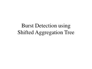
The exploration of burst detection using a Shifted Aggregation Tree (SAT) highlights its significance in efficiently identifying data bursts. This method introduces an Aggregation Pyramid (AP) structure, where nodes represent original data or aggregates, allowing for effective data visualization and comparison. The SAT algorithm systematically updates nodes and performs detailed searches within designated regions to ensure accurate detection of significant data patterns. This paper delves into the structure, benefits, and experimental validation of SAT, offering insights into its practical applications.

E N D
Content • Burst Detection Problem and Shifted Binary Tree • Aggregation Pyramid and Aggregation Tree • Shifted Aggregation Tree (SAT) and Detection Algorithm • Search for Best SAT Structure • Experiments and Discussion
Aggregation Pyramid (AP) • N-level pyramid-shape data structure built on a sliding window of length N • Level 1 has N cells containing original data, from left to right • Level 2 has N-1 cells, storing the aggregates for 2 consecutive data, i.e, a sliding sub-window of length 2 • Level h has N-h+1 cells, storing the aggregates for h consecutive data, i.e, a sliding sub-window of length h 12-level Aggregation Pyramid • Xin: Lots of double counting. This is not a generalization of SBT. (why having double counting can’t be a generalization? A SAT could be worse than SBT.)
Embed SBT in AP • Each node in Shifted Binary Tree is either an original data or an aggregate, which is a cell in Aggregation Pyramid, SBT can be embedded in AP. • Figure shows how each cell in SBT is embedded in the cell with the same color in AP. Embed SBT in AP
Aggregation Pyramid as Host Structure • Any structure composed of only aggregates and the original data can be embedded in AP. • It provides a host structure and a tool to visualize and compare different data structures. Another Embedded Structure
Aggregation Tree • A tree relation defined on a subset cells of Aggregation Pyramid containing all the first level cells • For any cell(t,h) in its domain, if cell(t,h) aggregates cell(t1,h1), cell(t2,h2)…cell(tn,hn), then cell(t,h) is the parent, cell(t1,h1) is the first child, …, cell(tn,hn) is the nth child. • Call cell(t,h) as node(t,k) if cell(t,h) is in the kth layer in the aggregation tree. Node(t,k) has the height of h in the aggregation pyramid, thus corresponds to a window of length h.
Notations The overlap of node(12,3) and node(16,3), i.e. cell(12,12) and cell(16,12), is cell(12,9), the dark gray cell.
Shifted Aggregation Tree (SAT) • Aggregation Tree w/ the following constraints (SAT Constraints) • Nodes in the same layer have the same sub-tree structure, i.e., if node(t,h) aggregates node(t1,h1), node(t2,h2), etc, node(t+s,h) aggregates node(t1+s,h1), node(t2+s,h2) and so on. All the children’s window lengths and relative orders in time are same, only shift in time. • Every node in the same layer shifts the same duration in time from its previous node. • The shift at layer l is a multiple of the shift at layer l-1. • The overlap window length of two adjacent nodes at layer l is greater than or equal to the window length at layer l-1
SAT Representation • Layer k can be represented by a triple (hk, sk, {ck1, ck2,…ckn}), where • hk, the corresponding level h in Aggregation Pyramid • sk, the shift, distance at layer 1 from leftmost leaf of node to the leftmost leaf of next node at same level. • {ckl, ck2, …ckn}, the layers for all its children • (hk, sk) in short when no confusion. • A SAT can be represented by a list of (hk, sk), the first triple represents the first layer and so on. • For example, {(1,1), (2,1), (4,2), (8,4)} represents a SWT of height 8
SAT Properties • The overlap window length owlk of two adjacent nodes at layer k is hk-sk • A window length h between hok-1 + 2 and hok +1 is always covered by a node at layer k
SAT Benefits • Structure not unique, defining a family of structures. • Variable (h,s) means variable bounding ratio T, controllable false alarm ratio and controllable detail search region. • Adaptive to the data!
Detection Algorithm w/ SAT • For each time point t, • start from layer 2, i.e., k=2 • while (a window ends) // need update node(t,k) (1) • update node(t,k) (2) • if node(t,k) exceeds the threshold of some length h in its Detail Search Region DSR(t,k) (3) • detail search DSR(t,k) Needs proof that you want to do this now. (4) • end • go to next layer, k ++
Detail Search Region (DSR) • DSR(t,k) : the region when node(t,k) updated, where to do detail search for real burst • A set of cells in aggregation pyramid within node(t,k)’s coverage • Exclude cells before t-sk which have been searched by node(t-sk,k), where sk is the shift at layer k • Exclude cells within DSR(t,k-1) which have been searched by node(t,k-1) Xin: I don’t understand this one. This may look for a different threshold. (Correct, for the whole coverage, you can do detail search, just not necessary if some part can be covered by lower nodes) • Loose DSR vs Tight DSR
Loose DSR • hok : the overlap window length of 2 adjacent nodes at layer k • A window length h between hok-1 + 2 and hok +1 is always covered by a node at layer k • A quadrilateral shape bounded by [t-sk+1, t] and [hk-1-sk-1+2, hk-sk+1] • Used by SBT
Tight DSR • A window length h between hok-1 + 2 and hk could be covered by a window hk , depending on the ending time • cell(t-1,hk-1) is covered by node(t,k), but cell(t-2, hk-1) is not • A m-nary fork shape, m=sk/sk-1 • For SBT, m=2, i.e, “L” shape • Has the same probability to raise an alarm as Loose DSR, but has less detail search cost on average, since some cells will be detected by a tight bound, especially with bound-&-prune detail search.
Naïve Detail Search • Search every cell in DSR one by one. • Cell(t+1,h+1)/cell(t-1/h-1) can be computed by adding/removing cell(t+1,1)/cell(t,1) from cell(t,h). • Starting from one seed cell, populate the whole interested DSR.
Grid-based Bound-&-Prune Detail Search • Given node(t,k), i.e., cell(t,hk), there are several cells at lower layershaving the same starting time or the same ending time. • By subtracting these cells, we can get some intermediate cells within DSR. • These cells form a grid and partition DSR. • Each cell has its own small DSR, if it doesn’t exceed the minimal threshold, no need to check its DSR. • Binary partition DSR, check big DSR first, then small DSR.
Grid-based Bound-&-Prune Detail Search • By subtracting a lower layer cell starting at the same time on the left, we can get a cell with the same color on the right. • The intermediate cells partitions the “L” shape tight DSR bounded by the red lines • cell(28,20) has its DSR bounded by the pink lines
Algorithm Complexity • Depend on specific SAT structure and the data to be detected • (Should have an analysis in the average case for the best SAT structure for the given data)
Search for Best SAT Structure • Given the above detection algorithm and the data to be detected, the best SAT structure minimizes the total running time. • Two major parts in the detection algorithm • updating the SAT structure, step (1) and (2) • detail searching DSR, step (3) and (4) • Best SAT structure balances between the updating time and the searching time.
Optimization Goal • The goal is to minimize • But how to quantitate the updating time and the searching time? • Theoretical method: estimate number of cell-access • Experiment method: count machine time on sample data
Estimate time by Number of Cell-access • Most part of the algorithm, i.e. step (2),(3),(4) are to access either the original data or an aggregate which is the same type as original data. • The number of cell-access implies how many operations are executed, thus an estimation of the running time. • Use the expected number of cell-access as the measurement of the expected running time. • Step (1) has the same number of execution as step (2), counted in step (2) by multiplying a weight learned from experiment.
Cell-access of node(t,l) • The updating step (2) requires to read all its children and write the aggregate to node(t,l), thus the number of cell-access is sizeof(children) + 1 • Step (3) can be done by a binary search to compare node(t,l) against the interested thresholds within DSR, requiring log2W+1 comparison, where W is the number of interested window lengths in this DSR.
Cell-access of node(t,l) (2) • For naïve detail search, to check one cell requires 4 cell-access (2 read, 1 write, 1 comparison against the threshold). • The probability to search a cell(t,h) is the probability to raise an alarm at level h given its covering node. Probalarm can be learned from sample data. • Total number of cell-access is
Time Cost of a SAT • Cost(SAT): • For theoretical method: • For experiment method: actual machine time to test on sample data with this SAT • Normalized Cost(SAT): • Where t is the total time points when counting or testing, and hL is the window length of the top layer • Comparable value for different SAT with different time cycles and different max window lengths • Best SAT is the one with minimal normalized cost which can cover the max interested window length N.
H-S grid as a search space • Map layer (h, s) to a grid cell in a regular h-s grid, origin at (1,1). • Link these grid cells by the SAT list order, a SAT can be mapped to a path in the h-s grid. • Shown two SAT paths • {(1,1)(3,3)(6,3)(12,3)} in red • {(1,1)(2,2)(4,2)(8,4)(12,4)} in blue • Grayed cells don’t satisfy SAT constraints, because h < s h-s grid and 2 SAT paths
Best SAT as shortest path • Any path ending above the line h-s+1=N, can at least cover window length N, thus no need for another layer. • Call the grid cells above the line h-s+1=N as final states, Best SAT is the shortest path starting from (1,1) to one of the final states and satisfying SAT constraints. • Multiple Single-Source-Shortest-Path (SSSP) problems between (1,1) and one of final states in a directed graph.
SSSP w/ Constraints • Not all the paths between (1,1) and a final state are legal, i.e, satisfying SAT constraints. • Unlimited final states, when to stop? • Large graph if considering all the possible edges between layer l-1 and layer l, many of them are not likely even in a good SAT, say {(1,1)(900,900)} is not likely in a SAT covering length 1000.
Best-first Graph Search • Best-first search in a dynamically-generated directed graph • Dynamically add edges to the graph for the node with best normalized cost • Guarantee all the paths are legal • Avoid to generate the unlikely edges • Stop searching after reaching M final states. • Dijastra-style cost update to track the shortest path • If the cost of a new path ending at current node is better than the cost kept in this node, update this node with the new cost
Search Algorithm • insert (1,1) into the graph and a heap based on the normalized cost • while the heap is not empty • pop the first node in the heap • if it’s a final node • if it’s already in the graph • if the new cost is better than the cost stored, update the cost • else insert the node into the graph and store its cost • if already reach M final nodes, stop • else • generate a set of next possible nodes for this node • for each next possible node • evaluate the normalized cost • if the new node is in the graph • If the new cost is better than the cost stored, update the cost • else insert the node into the graph and store its cost • insert this node into the heap • end while • output the best node and corresponding path with the best cost
Experiments • Test data: random normal-distributed N(6,1), 1M • Sample data: 20K • Interested windows are all the windows from length l up to the max length N • For window length h, the threshold Th is set to where bp is the real burst probability, is the normal cumulative function
SAT w/ naïve detail search vs SBT • Total running time in machine clock • SAT_EP: SAT found using experiment time cost • SAT_TH: SAT found using theoretical time cost • SBT: Shifted Binary Tree
Alarm probability is always large • In the testing data, even the real burst probability Probtrue is 0.0001, the probability for a window length l to exceed the threshold for length l-d, increases rapidly even d increases a little. • Figure right shows this probability for all the window length pairs less than 100 with Probtrue=0.0001. • When Probtrue is considerably large, updating time decides the SAT structure, since the detecting time are very close.
Discussion • SAT_EP is sensitive to CPU time, since it depends on the testing time on a small amount of sample data. Different runs may give different SAT structures. • It’s stable in the sense it always finds some SAT better than SBT. • SAT_TH doesn’t give an accurate estimation of actual running time. • But when Probalarm is large, it produces better comparison of updating cost between different SAT, thus better result.
SAT w/ naïve detail search vs SBT (3) • Breakdown time in machine clock for SAT_EP