 sd = solar diffuser scan angle = Band Avg. SD screen transmittance

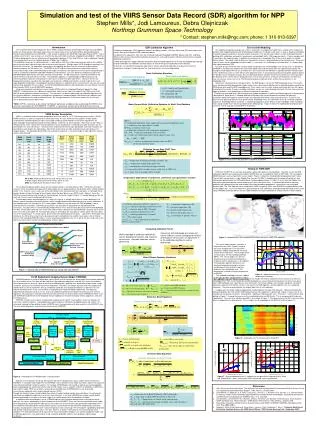
1. 280 275 ElectronicsTemperature (K) 270 thermst #11 thermst #12 265 thermst #13 thermst #14 thermst #15 thermst #16 thermst #17 thermst #18 260 True Temp 255 0 0.1 0.2 0.3 0.4 0.5 0.6 0.7 0.8 0.9 1.0 Fraction of Orbit Simulation and test of the VIIRS Sensor Data Record (SDR) algorithm for NPP Stephen Mills*, Jodi Lamoureux, Debra Olejniczak Northrop Grumman Space Technology * Contact: stephen.mills@ngc.com; phone: 1 310 813-6397 Introduction The Visible/Infrared Imager Radiometer Suite (VIIRS), built by Raytheon Santa Barbara Remote Sensing (SBRS) will be one of the primary earth-observing remote-sensing instruments on the National Polar-Orbiting Operational Environmental Satellite System (NPOESS). It will also be installed on the NPOESS Preparatory Project (NPP). These satellite systems fly in near-circular, sun-synchronous low-earth orbits at altitudes of approximately 830 km. VIIRS has 15 bands designed to measure reflectance with wavelengths between 412 nm and 2250 nm, and an additional 7 bands measuring primarily emissive radiance between 3700nm and 11450 nm. The calibration source for the reflective bands is a solar diffuser (SD) that is illuminated once per orbit as the satellite passes from the dark side to the light side of the earth near the poles. Sunlight enters VIIRS through an opening in the front of the instrument. An attenuation screen covers the opening, but other than this there are no other optical elements between the SD and the sun. The BRDF of the SD and the transmittance of the attenuation screen is measured pre-flight, and so with knowledge of the angles of incidence, the radiance of the sun can be computed and is used as a reference to produce calibrated reflectances and radiances. Emissive bands are calibrated using an on-board blackbody (BB) that has also been carefully characterized. The BB temperature is carefully controlled using heater elements and thermistors in the BB. The calibration algorithm, using knowledge of BB temperature and emissivity, predicts radiances and compares it with counts to determine gain adjustments. Because of emissive background variations caused by the half-angle scanning mirror, additional corrections must be made for this scan-angle dependent modulation. Knowledge of spacecraft ephemeris, alignment errors and instrument scan rate are used to accurately geolocate the sensor data. The combined calibrated radiances with geolocation are referred to as Sensor Data Records (SDR) in the NPOESS/NPP program. Using environmental and radiative transfer models (RTM) within the Integrated Weather Products Test Bed (IWPTB)*, simulated earth view radiances are generated, and these are input into model of the VIIRS sensor in the IWPTB, which produces simulated raw counts. The raw counts are processed through the calibration algorithm and the resultant radiances, reflectances and brightness temperatures compared against the known truth radiances from the RTM to determine the residual calibration error. By varying parameters in the sensor model, the sensitivity of sensor performance can be determined. *Note: IWPTB is referred to as Environmental Products Verification and Remote Sensing Testbed (EVEREST) when not used in conjunction with NPOESS/NPP. EVEREST is a proprietary software tool of Northrop Grumman Corp. • SDR Calibration Algorithm • Radiometric calibration (SDR) algorithms convert raw digital numbers (DN) from Earth View (EV) observations into various Sensor Data Record (SDR) radiance products. • As part of these algorithms, DNs from the On-Board Calibrator Blackbody (OBCBB), Space View (SV), and Solar Diffuser (SD) view are adjusted for background signal levels and used to update reflective band and emissive band calibration coefficients. • VIIRS SDR algorithms apply calibration coefficients determined during pre-launch testing and updated operationally through calibration and validation (cal/Val) analysis to transfer the ground calibration to on-orbit data. • Provisions are included to incorporate adjustments into the radiometric calibration to account for instrument temperature, changes in incoming solar flux, and to correct for instrument degradation. • Basic Calibration Equations • Basic Second Order Calibration Equation for Earth View Radiance • Emission Versus Scan (EVS) Term • Temperature dependence of calibration coefficients uses parametric function • Computing Calibration Factor • Solar Diffuser Geometry Equations • Reflective Band Equations • Emissive Band Equations Error & Drift Modeling For modeling temporally varying errors, there is a common shared generic model that is used by all the modules to produce time-stepped realization with temporally correlated error. It includes static errors as well as temporal oscillations at specific frequency and phase and also random-walk errors. The generic error model is used to model pointing jitter, pointing drifts, calibration source drifts, band center and bandwidth drifts, FPA temperature drifts, 1/f noise and gain drift. In each case, the model includes, in addition to the actual error, a knowledge filter of the system, which can include latency effects. The model is able to determine how well the system is able to compensate a particular error. There are 3 types of errors that are produced in the drift model: 1). static error; 2). oscillating or sinusoidal error; 3). random-walk error represented by a PSD. For each of these three the error is broken down into design error and knowledge error. Design error, as defined for VIRRISM, is the difference between the nominal designed value and the actual value for a particular parameter. For example, the designed nominal axis of rotation for a crosstrack scan (whiskbroom) is typically along the velocity vector of the satellite, but of course, there will be some alignment errors in manufacturing and mounting which would be part of the design error for roll, pitch and yaw. Tests are done both before and after launch to characterize as well as possible the deviation of the system from its designed values. These measurements, of course are not perfect, and they also may not measure some errors at all. The difference between the design errors and the measured errors is the knowledge error. Static error is defined with just two parameters--the RMS design error and the RMS knowledge error. In the model these are determined by drawing two random values from a Gaussian distribution with a standard deviation equal to the RMS design error and the RMS knowledge error. These values are truly static, and do not change with time for a given realization of the model. Of course, multiple realizations can be run, and evaluated statistically. For the static errors that apply to detectors, each detector gets a different independent realization. Oscillating or sinusoidal errors do not include any random component. A specific oscillating frequency is defined with a specific phase. Since phase is included, different oscillating errors can be temporally correlated. For pointing, oscillations would correspond to specific modes that would be determined using structural analysis. Of course, the phase of yaw, pitch and roll errors may be correlated. Knowledge errors are specified in terms of oscillation amplitude and phase. Knowledge latency, therefore, is modeled by applying a phase delay in to the knowledge. Other oscillating errors could include errors that are correlated to the orbital period. Figure 3 shows the modeled drift of detector dark current (1/f noise) and gain for band M16 for 5 detectors. Figure 3 – Dark current and gain drifts modeled for band M16 Planck black body radiance Relative Spectral Response • fix() = end-to-end transmittance •  = wavelength (microns) • T = temperature (K) • QE = quantum efficiency Definition of band averaging VIIRS Sensor Description VIIRS is a visible/infrared instrument designed to satisfy the needs of 3 U. S. Government communities—NOAA, NASA and DOD, as well as the general research community. As such, VIIRS has key attributes of high spatial resolution with controlled growth off nadir, and a large number of spectral bands to satisfy the requirements for generating high quality operational and scientific products. VIIRS has 22 spectral bands, 15 of which are classified as reflective bands, that is, bands where the predominant source of radiances is reflected solar light, and which are all wavelengths less than 2.5 microns. Nominal values of band center wavelength, band width, and nadir resolution are described for each band in the table below. Note that 5 of the bands are high resolution bands referred to as the imagery bands. The Day/Night Band (DNB) has a dynamic range that is sensitive enough to allow nighttime moon lit scenes to be detected. M1 to M16: Moderate Resolution bands 750 by 750 m at nadir I1 to I5: Imagery Resolution bands 375 by 735 m at nadir DNB: Day Night Band, Resolution 750 by 750 m The On-Board Calibrator (OBC) source for the reflective bands is the Solar Diffuser (SD). VIIRS views the earth using a 3-mirror anastigmat telescope which rotates about an axis approximately in the direction of the satellite velocity vector. Thus, it paints a cross-track scan of the earth below itself, and centered at the nadir point. A half-angle mirror counter-rotates to relay the image to the aft-optics where the focal plane arrays (FPA) reside. Figure 1 shows the VIIRS instrument cutaway view through the front bulkhead. The center image in Figure 1 is viewed looking up from the earth with the instrument moving toward the viewer. The telescope rotates counterclockwise (as seen in this figure), it sweeps left to right as it faces downward, first taking a space view above the earth’s horizon, which is used to determine the dark counts to be used in calibration. It then sweeps across the earth over a 112 swath (approx. 3000 km), then up across the OBC blackbody used to calibrate the emissive bands, and finally up and across the solar diffuser attached to the top bulkhead of the instrument. The solar diffuser is illuminated by sunlight when it shines into the solar diffuser port on the front bulkhead of VIIRS. The SD port cannot be seen in the main view in Figure 1 because the front bulkhead is cutaway, but it can be seen in the view in the upper left. The solar diffuser port is covered by the solar diffuser screen, which transmits about 12% of the incident light. It is made up of a grid of small holes drilled about 2 mm apart. Light enters the SD port and illuminates the SD for only a few minutes during each orbit, shortly before the satellite moves across the terminator. For the 1730 ascending NPOESS orbit, it is never fully illuminated because the sun is too far off to the side, and so this orbit must rely on other methods of calibrating the reflective bands. Figure 1 - Cutaway view of VIIRS showing scan cavity, with solar diffuser Dark current change (A x 10-12) 200 1/f noise (dark current drift) Where F = calibration adjustment factor, updated from on-board calibration source ev = earth view scan angle relative to nadir RVS(ev) = response versus scan ci = calibration coefficients with temperature dependence DNev, DNsv= earth view and space view raw counts dnev= earth view differential counts which subtracts space view 0 -200 6 Gain Change x 10-4 Gain drift 0 Lbkg(ev)= emissive background variation with scan (EVS) = 0 for non-emissive bands. -6 -12 0 20 40 60 • Trta = temperature of rotating telescope assembly (K) • Tham = temperature of half-angle mirror (K) • rta = transmittance of rotating telescope assembly •  = scan angle relative to nadir, may be earth view or OBC view • sv = space view scan angle relative to nadir Testing of VIIRS SDR RTM from the IWPTB runs too slow to produce a whole orbit worth of simulated data. Therefore, to test the SDR calibration algorithm for a large amount of data, MODIS data was resampled to match an NPP orbit. This resampled MODIS data was used as input to the sensor model. Figure 4 shows the simulated orbit and projected earth scene. The test data was based on a single Golden Day, January 25, 2003 It modeled realistic spacecraft ephemeris and attitude data generated for the NPP orbital plane, Produced approximately 1.2 orbits (2 hours) from the Golden Day, with perfect spacecraft attitude control assumed (roll, pitch, yaw set to zero) . It combined the sensor’s scanning geometry with spacecraft position and attitude information to produce geolocated sensor pixels and associated auxiliary data. The TOA radiances were emulated for VIIRS using proxy SDRs from MODIS on the Aqua platform and for the Golden Day. The sensor model then generated Earth-view, calibration, and engineering RDR data for the sensor using VIRRISM consistent with the sensor’s SDR software. Test data restricted to a limited number of sensor effects. ration algorithm is essentially the inverse of the sensor model, the residual radiometric errors mostly result from this knowledge error. The sensor model was used to produced raw sensor data containing counts for earth view, space view, OBC blackbody view, solar diffuser view, thermistors, DC restore voltage, scan encoder, along with simulated ephemeris data from the satellite. All this is the input to the SDR algorithm, and the algorithm was run, outputting radiances. These were compared with the original input files of truth radiances. In appearance the output radiance appeared to exactly duplicate the input truth radiance. However, by taking the difference between the truth and the SDR output the error in the algorithm is determined. Figure 6 shows error for an example on one granule (16 scans) for band M15. Significant striping can be seen. The error is sorted into bins and plotted in Figure 7, showing the mean error the standard deviation and RMS error. This is compared with the design specification. The error for a reflective band M3 is also shown in Figure 7. The dominant error for M3 is the mean error, which is proportional to radiance level. This is largely due to knowledge of the BRDF of the SD of about 1%. Where = Radiance per photoelectron • G =Electro-optic gain in W/(m2sr micron e-) • a1(Tdet) = effective capacitance of detector (e-/V) • b1(Telec) = Inverse gain of ADC (V/count) • a2(Tdet)= capacitace nonlinearity (e-/V2) • b2(Telec) = Analog nonlinearity (V/count2) • Vdcr = DC restore signal • ci(Tdet,Telec) = delta adjustment to calibration W/(m2sr micron counti) • Telec = electronics temperature (K) • Tdet= detector temperature (K) • A = detector field stop area (m) • t = detector integration time (s) • stop= solid angle of aperture stop (sr) Conversely with knowledge of a known cal source radiance, counts, background variation and response versus scan, an adjustment, F, to the calibration coefficients can be determined With knowledge of calibration coefficients, counts, background variation and response versus scan, unknown radiances can be determined Figure 4 – Modeled orbit & Resampled MODIS data used to test VIIRS SDR algorithm The sensor model includes variations in temperature over orbit. Figure 5 shows 6 thermistor temperatures in or around the electronics module along with the true temp-erature of the electronics. These temperatures are based on a thermal model provided by SBRS. The sensor model uses the true temperature to vary electronic temperature response, but this temperature is not reported. The calibration algorithm determines the electronic temperature based on a linear combination of the thermistors and thus produces some knowledge error. This temperature is called instrument temperature on MODIS. The modeled knowledge error was applied to the look-up tables and parameters used by the calibration algorithm. Since the SDR calib- Figure 5 – Modeled thermistors used for electronics temperature estimation Vis/IR Radiometric Imaging Sensor Model (VIRRISM) VIRRISM produces a stream of digital data, which can be used to simulate the actual output that would be produced by a real remote sensor. This data can be used to test the calibration algorithms used with the sensor and evaluate sensor performance in terms of signal-to-noise ratio, calibration bias, pointing error, band-to-band registration, image resolution, spectral error environmental retrieval algorithms. Therefore, the model is dynamic and time stepped, and includes drifts in sensor parameters that are temporally, spectrally and spatially correlated. It is able to assess the effect of correlated errors in the sensor, which an expected value model would be unable to do. The impact on radiometric performance can be assesses, and since radiometric performance affects the performance of retrieval algorithms, the accuracy of retrieved environmental measurements can also be determined. VIRRISM has been used with EVEREST to determine end-to-end performance modeling for environmental data retrieval algorithms used with the VIIRS sensor. VIRRISM simulates most aspects of radiometric imaging sensors within 7 sub-modules. These are modules for noise, bias, spectral response, scanning/pointing, spatial response, electronics and digital processing. Figure 2 is a schematic showing the flow of data through VIRRISM and its interconnection with other models in the EVEREST suite. The cyan and yellow boxes show elements that are part of VIRRISM. Figure 2 - Flow diagram of VIRRISM and its interconnections Note the sensor database at the top. Data can be fed into this database by various models that are external to EVEREST. It should be understood here that VIRRISM is not a detailed sensor model, but rather, requires the output of more detailed modeled in order to function. For example, VIRRISM does not include an optical ray-tracing capability, but instead depends on commercial off-the-shelf (COTS) models such as codeV, OSLO or ZEMAX or NGST’s in-house optics model, PRG, any of which can provide the detailed data to VIRRISM that it uses to describe transmittance, alignment errors or point spread functions (PSF). Though the flowchart shows simulated data from external models feeding into the sensor database, this data could alternately be supplied through tests and system measurements. In this way VIRRISM can also be used to predict performance based on test data at the later stages in a satellite project when this becomes available. In addition to data describing the sensor, VIRRISM requires the simulated radiance values entering the sensor aperture. This data is produced by 3 other components of the EVEREST Suite: the Earth environmental scene model, the orbital geometry model and the radiative transfer model. The environmental scene generation model determines the conditions of the atmosphere and the Earth’s surface. This includes the atmosphere’s temperatures, pressures, humidity, cloud properties and the Earth surface temperature and surface type. The atmosphere is gridded by longitude and latitude, and by elevation into layers. This data, taken as a whole, is referred to as the environmental scene database. The atmospheric data can be input from a measured weather database, or a weather prediction model such as MM5 can generate it. The advantage of using a weather prediction model is that it produces higher spatial resolution. • v= SD screen vertical angle, • h= SD screen horizontal angle, • inc= SD angle of incidence with respect to normal • inc= SD azimuthal angle incidence • sinst = Solar vector WRT instrument • ssd = Solar vector WRT SD normal • Tsd/inst = Transformation matrix from instrument to SD coordinates Radiance on Solar Diffuser (SD) Calibration Factor Drift/Error Model Static i Random Walk i Oscillatory External Models Pointing Errors & Jitter Band Center & BW Errors Linear & Nonlinear Response Drift Linear & Nonlinear Electronic Drift Reflectance Coefficients Calibrated Earth Reflectance Digital Counts (RDR) Pointing & Blurring Model Spectral (filtering) Model Detector Response & Noise Model Electronic Response & ADC Model RTM Radiance Volts noise & flux Blurred spectral radiance Blurred radiance Point Spread function Optics Model (code V) Figure 6 – Calibration error for one granule for Band M15 • dse= Sun to earth distance • = annually average dse • = annually averaged solar irradiance • = Band-averaged BRDF of SD • sd= solar diffuser scan angle • = Band Avg. SD screen transmittance • sun_earth= solar zenith angle on earth (from geolocation) Background Irradiance Aggregation B2B Misregistration To Cal Alg Compute Emissive Background Calib. radiance RVS Scan BRDF Error & Drift M15 M3 Detector Temp Electronic Temp Background Temperatures Error (W/(m2sr micron)) Error (W/(m2sr micron)) Calibration Model Space View i Solar Diffuser i Blackbody Thermal Model Drift/Error i Orbital (from SBRS) i Thermistors Emissive Calibration Correction Factor Model Products/knobs External IWPTB Models/Tools Sensor Model Modules Radiance (W/(m2sr micron)) Radiance (W/(m2sr micron)) Figure 7 – Binned calibration error vs. radiance for one granule for Band M3 & M15. Solid red, Standard Dev.; green, mean; blue, RMS; dashed red, sensor specification. Reflected Emissive Radiance off On-Board Calibration Black Body • References • Hal J. Bloom and Peter Wilczynski, “The National Polar-orbiting Operational Environmental Satellite System: Future U.S. Operational Earth Observation System”, ITSC XIII Proc., October 2003 • Carol Welsch, H. Swenson, S. A. Cota, F. DeLuccia, J. M. Hass, C. Schueler, R. M. Durham, J. E. Clement and P. E. Ardanuy, “VIIRS, A Next Generation Operational Environmental Sensor for NPOESS,” International Geoscience and Remote Sensing Symposium (IGARSS) Proc., 8-14, July 2001. • Carl Schueler, J. Ed Clement, Russ Ravella, Jeffery J. Puschell, Lane Darnton, Frank DeLuccia, Tanya Scalione USAF, Hal Bloom and Hilmer Swenson, “VIIRS Sensor Performance,” ITSC XIII Proc., October 2003 • Steve Mills, “Simulation of Earth Science Remote Sensors with NGST's EVEREST/VIRRISM, AIAA Space 2004 Conf. Proc. 5954 (2004) • Stephen P. Mills, Hiroshi Agravante, Bruce Hauss, James E. Klein, Stephanie C. Weiss, “Computer Modeling of Earthshine Contamination on the VIIRS Solar Diffuser,” SPIE Remote Sensing Conf., September 2005 • obc= Emission of On-Board Calibrator (OBC) black body • obc= Scan angle at which OBC black body is observed • Tsh, Tcav, Ttele = Temperatures of shield, cavity and telescope • Fsh, Fcav, Ftele = Fractional solid angle of shield, cavity and telescope as reflected onto OBC black body