Two Factor Designs
BRAND. 1 2 3 4 17.9, 18.1 17.8, 17.8 18.1, 18.2 17.8, 17.9 18.0, 18.2 18.0, 18.3 18.4, 18.1 18.1, 18.5 18.0, 17.8 17.8, 18.0 18.1, 18.3 18.1, 17.9. 1 2 3. DEVICE. Two Factor Designs. Consider studying the impact of two factors on the yield (response):. NOTE: The “1”, “2”,etc...

Two Factor Designs
E N D
Presentation Transcript
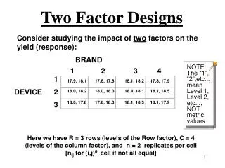
BRAND 1 2 3 4 17.9, 18.117.8, 17.818.1, 18.217.8, 17.9 18.0, 18.218.0, 18.318.4, 18.118.1, 18.5 18.0, 17.817.8, 18.018.1, 18.318.1, 17.9 1 2 3 DEVICE Two Factor Designs Consider studying the impact of two factors on the yield (response): NOTE: The “1”, “2”,etc... mean Level 1, Level 2, etc..., NOT metric values Here we have R = 3 rows (levels of the Row factor), C = 4 (levels of the column factor), and n = 2 replicates per cell [nij for (i,j)th cell if not all equal]
MODEL: Yijk = ijijijk i = 1, ..., R j = 1, ..., C k= 1, ..., n In general, n observations per cell, R • C cells.
:the grand mean • i: the difference between the ith • row mean and the grand mean • j : the difference between the jth • column mean and the grand mean • ij : the interaction associated with • the i-th row and the j-th column (= ij -i-j- )
Yijk = Y•••+ (Yi•• - Y•••) + (Y•j• - Y•••) + (Yij• - Yi•• - Y•j• + Y•••) + (Yijk - Yij•) Where Y•••= Grand mean Yi••= Mean of row i Y•j•= Mean of column j Yij•= Mean of cell (i,j) [All the terms are somewhat “intuitive”, except for (Yij• -Yi•• -Y•j• + Y•••)]
The term (Yij• -Yi•• -Y•j• + Y•••) is more intuitively written as: (Yij• - Y•••) (Yi•• - Y•••) (Y•j• - Y•••) adjustment for “row membership” adjustment for “column membership” how a cell mean differs from grand mean We can, without loss of generality, assume (for a moment) that there is no error (random part); why then might the above be non-zero?
BL BH AL 5 8 AH 10 ? “INTERACTION” ANSWER: Two basic ways to look at interaction: 1) If AHBH = 13, no interaction If AHBH > 13, + interaction If AHBH < 13, - interaction - When B goes from BLBH, yield goes up by 3 (58). - When A goes from AL AH, yield goes up by 5 (510). - When both changes of level occur, does yield go up by the sum, 3 + 5 = 8? Interaction = degree of difference from sum of separate effects
BL BH AL 5 8 AH 10 17 2) - Holding BL, what happens as A goes from ALAH? +5 - Holding BH, what happens as A goes from AL AH? +9 If the effect of one factor (i.e., the impact of changing its level) is DIFFERENT for different levels of another factor, then INTERACTION exists between the two factors. NOTE: - Holding AL, BL BH has impact + 3 - Holding AH, BL BH has impact + 7 (AB) = (BA) or (9-5) = (7-3).
Going back to the (model) equation on page 4, and bringing Y... to the other side of the equation, we get (Yijk - Y•••) = (Yi•• - Y•••) + (Y•j• - Y•••) + [(Yij• - Yi••) - (Y•j• - Y•••)] + (Yijk - Yij•) Effect of column j at row i. Effect of column j If we then square both sides, triple sum both sides over i, j, and k, we get, (after noting that all cross-product terms cancel):
(Yijk - Y•••)n.C.Yi•• - Y••• i j k i + n.R.Y•j• - Y•••)2 + n.Yij• - Yi•• - Y•j• +Y••• i j (Yijk - Yij• i j k TSS = SSBRows + SSBCols+ SSIR,C+ SSWError and, in terms of degrees of freedom, R.C.n-1 = (R-1) + (C-1) + (R-1)(C-1) + R.C.(n-1); DF of Interaction = (RC-1)-(R-1)-(C-1) = (R-1)(C-1). j OR,
1 2 3 BRAND In our example: 1 2 3 4 17.9, 18.117.8, 17.818.1, 18.217.8,17.9 18.117.818.1517.85 18.2, 18.018.0, 18.318.4, 18.118.1, 18.5 18.118.1518.2518.3 18.0, 17.817.8, 18.018.1, 18.318.1, 17.9 17.917.918.218.0 17.95 D E V I C E 18.20 18.00 18.05 18.00 17.95 18.20 18.05
SSBrows =2 4[(17.95-18.05) 2 + (18.20-18.05) 2 + (18.0-18.05) 2] = 8 (.01 + .0225 + .0025) = .28 SSBcol =2•3[(18-18.05) 2+(17.95-18.05) 2+(18.2-18.05) 2+( 18.05-18.05) 2] = 6 (.0025 + .001 + .0225 + 0) = .21 SSIR,C = 2 • [ • (18-17.95-18+18.05)2 + (17.8-17.95-17.95+18.05)2 ....… + (18-18-18.05+18.05)2 ] = 2 [.055] = .11 SSW = (17.9-18.0) 2 + (18.1-18.0) 2 + (17.8-17.8) 2 + (17.8-17.8) 2 + … ....... (18.1-18.0) 2 + (17.9-18.0) 2 = .30 TSS = .28 + .21+ .11 + .30 = .90
SOURCE SSQ df M.S. Fcalc Rows .28 2 .14 5.6 COL .21 3 .07 2.8 Int’n .11 6 .0183 .73 Error .30 12 .025 ANOVA .05 1) Ho: All Row Means Equal H1: Not all Row Means Equal 2) Ho: All Col. Means Equal H1: Not All Col. Means Equal 3) Ho: No Int’n between factors H1: There is int’n between factors FTV (2, 12) = 3.89 Reject Ho FTV (3, 12) = 3.49 Accept Ho FTV (6, 12) = 3.00 Accept Ho
An issue to think about: We have: E ( MSI) =+ Vint’n E (MSW) = Since Vint’n cannot be negative, and MSI = .0183 < MSW = .025, some argue that this is “strong” evidence that Vint’n is not > 0. If this is true, E(MSI) = , and we should combine MSI and MSW (i.e., “pool”) estimates. This gives: SSQdfMS SSQdfMS Int. .11 6 .0183 Error .41 18 .0228 Error .30 12 .025 to (Some stat packages suggest what you should do).
Another issue: The table of 2 pages ago assumes what is called a “Fixed Model”. There is also what is called a “Random Model” (and a “Mixed Model”). MEAN SQUARE EXPECTATIONS col = fixed row= random Fixed Random Mixed MSBrows + VR + VI+VR+ VR MSBcol + VC+ VI+VC+ VI+ VC MSBInt’n + VI+ VI+ VI MSWerror Reference: Design and Analysis of Experiments by D.C. Montgomery, 4th edition, Chapter 11.
Fixed: Specific levels chosen by the experimenter Random: Levels chosen randomly from a large number of possibilities Fixed: All Levels about which inferences are to be made are included in the experiment Random: Levels are some of a large number possible Fixed: A definite number of qualitatively distinguishable levels, and we plan to study them all, or a continuous set of quantitative settings, but we choose a suitable, definite subset in a limited region and confine inferences to that subset Random: Levels are a random sample from an infinite ( or large) population
“In a great number of cases the investigator may argue either way, depending on his mood and his handling of the subject matter. In other words, it is more a matter of assumption than of reality.” Some authors say that if in doubt, assume fixed model. Others say things like “I think in most experimental situations the random model is applicable.” [The latter quote is from a person whose experiments are in the field of biology].
My own feeling is that in most areas of management, a majority of experiments involve the fixed model [e.g., specific promotional campaigns, two specific ways of handling an issue on an income statement, etc.] . Many cases involve neither a “pure” fixed nor a “pure” random situation [e.g., selecting 3 prices from 6 “practical” possibilities]. Note that the issue sometimes becomes irrelevant in a practical sense when (certain) interactions are not present. Also note that each assumption may yield you the same “answer” in terms of practical application, in which case the distinction may not be an important one.
Brand Name Appeal for Men & Women: M F Interesting Example:* Frontiersman April 50 people per cell Mean Scores “Frontiersman” “April” “Frontiersman” “April” Dependent males males females females Variables (n=50) (n=50) (n=50) (n=50) Intent-to- purchase 4.44 3.50 2.04 4.52 (*) Decision Sciences”, Vol. 9, p. 470, 1978
ANOVA Results Dependent Source d.f. MS F Variable Intent-to- Sex (A) 1 23.80 5.61* purchase Brand name (B) 1 29.64 6.99** (7 pt. scale) A x B 1 146.21 34.48*** Error 196 4.24 *p <.05 **p <.01 ***p <.001
Two-Way ANOVA in Minitab Stat>>Anova>>General Linear Model: Model device brand device*brand device Random factors Tick “Display expected mean squares and variance components” Results Factor plots Main effects plots & Interactions plots Graphs Use standardized residuals for plots
Two Factors with No Replication, A 1 2 3 1 7 3 4 2 10 6 8 3 6 2 5 4 9 5 7 B When there’s no replication, there is no “pure” way to estimate ERROR. Error is measured by considering more than one observation (i.e., replication) at the same “treatment combination” (i.e., experimental conditions).
Our model for analysis is “technically”: Yij = i j + Iij i = 1, ..., R j = 1, ..., C We can write: Yij = Y•• + (Yi• - Y••) + (Y•j - Y••) + (Yij - Yi• - Y•j+ Y••)
After bringing Y•• to the other side of the equation, squaring both sides, and double summing over i and j, We Find: Yij - Y••)2 = C • Yi•-Y••)2 + R • Y•j - Y••)2 + (Yij - Yi• - Y•j + Y••)2 R C R j=1 i=1 i = 1 C j=1 R C j=1 i=1
TSS = SSBROWS + SSBCol + SSIR, C Degrees of Freedom : R•C - 1 = (R - 1) + (C - 1) + (R - 1) (C - 1) We Know, E(MSInt.) = VInt. If we assumeVInt. = 0, E(MSInt.) = 2, and we can call SSIR,C SSW MSInt MSW
And, our model may be rewritten: Yij = + i + j + ij, and the “labels” would become: TSS = SSBROWS+ SSBCol + SSW Error In our problem: SSBrows = 28.67 SSBcol = 32 SSW = 1.33
and: ANOVA Fcalc df Source SSQ MSQ at = .01, FTV (3,6) = 9.78 FTV(2,6) = 10.93 28.67 32.00 1.33 rows col Error 9.55 16.00 00.22 3 2 6 43 72 TSS = 62 11
What if we’re wrong about there being no interaction? If we “think” our ratio is, in Expectation, 2 + VROWS , (Say, for ROWS) 2 and it really is (because there’s interaction) 2 + VROWS, 2 + Vint’n being wrong can lead only to giving us an underestimated Fcalc.
Thus, if we’ve REJECTED Ho, we can feel confident of our conclusion, even if there’s interaction If we’ve ACCEPTED Ho, only then could the no interaction assumption be CRITICAL.
Blocking • We will add a factor even if it is not of interest so that • the study of the prime factors is under more homogeneous • conditions.This factor is called “block”. Most of time, the • block does not interact with prime factors. • Popular factors are “location”, “gender” and so on. • A two-factor design with one block factor is called a • “randomized block design”.
For example, suppose that we are studying worker absenteeism as a function of the age of the worker, and have different levels of ages: 25-30, 40-55, and 55-60. However, a worker’s gender may also affect his/her amount of absenteeism. Even though we are not particularly concerned with the impact of gender, we want to ensure that the gender factor does not pollute our conclusions about the effect of age. Moreover, it seems unlikely that “gender” interacts with “ages”. We include “gender” as a block factor.