Parallel Computing 2007: Science Applications

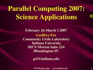
Parallel Computing 2007:Science Applications February 26-March 1 2007 Geoffrey Fox Community Grids Laboratory Indiana University 505 N Morton Suite 224 Bloomington IN gcf@indiana.edu PC07ScienceApps gcf@indiana.edu

Four Descriptions of Matter -- Quantum, Particle, Statistical, Continuum • Quantum Physics • Particle Dynamics • Statistical Physics • Continuum Physics • These give rise to different algorithms and in some cases, one will mix these different descriptions. We will briefly describe these with a pointer to types of algorithms used. • These descriptions underlie several different fields such as physics, chemistry, environmental modeling, climatology. • indeed any field that studies physical world from a reasonably fundamental point of view. • For instance, they directly underlie weather prediction as this is phrased in terms of properties of atmosphere. • However, if you simulate a chemical plant, you would not phrase this directly in terms of atomic properties but rather in terms of phenomenological macroscopic artifacts - "pipes", "valves", "machines", "people" etc. (today several biology simulations are of this phenomenological type) • General Relativity and Quantum Gravity • These describe space-time at the ultimate level but are not needed in practical real world calculations. There are important academic computations studying these descriptions of matter. PC07ScienceApps gcf@indiana.edu

Quantum Physics and Examples of Use of Computation • This is a fundamental description of the microscopic world. You would in principle use it to describe everything but this is both unnecessary and too difficult both computationally and analytically. • Quantum Physics problems are typified by Quantum Chromodynamics (QCD) calculations and these end up looking identical to statistical physics problems numerically. There are also some chemistry problems where quantum effects are important. These give rise to several types of algorithms. • Solution to Schrodinger's equation (a partial differential equation). This can only be done exactly for simple 2-->4 particle systems • Formulation of a large matrix whose rows and columns are the distinct states of the system. This is followed by typical matrix operations (diagonalization, multiplication, inversion) • Statistical methods which can be thought of as Monte Carlo evaluation of integrals gotten in integral equation formulation of problem • These are Grid (QCD) or Matrix PC07ScienceApps gcf@indiana.edu

Particle Dynamics and Examples of Use of Computation • Quantum effects are only important at small distances (10-13 cms for the so called strong or nuclear forces, 10-8 cm for electromagnetically interacting particles). • Often these short distance effects are unimportant and it is sufficient to treat physics classically. Then all matter is made up of particles - which are selected from set of atoms (electrons etc.). • The most well known problems of this type come from biochemistry. Here we study biologically interesting proteins which are made up of some 10,000 to 100,000 atoms. We hope to understand the chemical basis of life or more practically find which proteins are potentially interesting drugs. • Particles each obey Newton's Law and study of proteins generalizes the numerical formulation of the study of the solar system where the sun and planets are evolved in time as defined by Gravity's Force Law PC07ScienceApps gcf@indiana.edu

Particle Dynamics and Example of Astrophysics • Astrophysics has several important particle dynamics problems where new particles are not atoms but rather stars, clusters of stars, galaxies or clusters of galaxies. • The numerical algorithm is similar but there is an important new approach because we have a lot of particles (currently over N=107) and all particles interact with each other. • This naively has a computational complexity of O(N2) at each time step but a clever numerical method reduces it to O(N) or O (NlogN). • Physics problems addressed include: • Evolution of early universe structure of today • Why are galaxies spiral? • What happens when galaxies collide? • What makes globular clusters (with O(106) stars) like they are? PC07ScienceApps gcf@indiana.edu

Statistical Physics and Comparison of Monte Carlo and Particle Dynamics • Large systems reach equilibrium and ensemble properties (temperature, pressure, specific heat, ...) can be found statistically. This is essentially law of large numbers (central limit theorem). • The resultant approach moves particles "randomly" asccording to some probability and NOT deterministically as in Newton's laws • Many properties of particle systems can be calculated either by Monte Carlo or by Particle Dynamics. Monte Carlo is harder as cannot evolve particles independently. • This can lead to (soluble!) difficulties in parallel algorithms as lack of independence implies that synchronization issues. • Many quantum systems treated just like statistical physics as quantum theory built on probability densities PC07ScienceApps gcf@indiana.edu

Continuum Physics as an approximation to Particle Dynamics • Replace particle description by average. 1023 molecules in a molar volume is too many to handle numerically. So divide full system into a large number of "small" volumes dV such that: • Macroscopic Properties: Temperature, velocity, pressure are essentially constant in volume • In principle, use statistical physics (or Particle Dynamics averaged as "Transport Equations") to describe volume dV in terms of macroscopic (ensemble) properties for volume • Volume size = dV must be small enough so macroscopic properties are indeed constant; dV must be large enough so can average over molecular motion to define properties • As typical molecule is 10-8 cm in linear dimension, these constraints are not hard • Breaks down sometimes e.g. leading edges at shuttle reentry etc. Then you augment continuum approach (computational fluid dynamics) with explicit particle method PC07ScienceApps gcf@indiana.edu

Computational Fluid Dynamics • Computational Fluid Dynamics is dominant numerical field for Continuum Physics • There are a set of partial differential equations which cover • liquids including blood, oil etc. • gases including airflow over wings and weather • We apply computational "fluid" dynamics most often to the gas - air. Gases are really particles • If a small number (<106) of particles, use "molecular dynamics" and if a large number (1023) use computational fluid dynamics. PC07ScienceApps gcf@indiana.edu

Computational Sweet Spots • A given application needs a certain computer performance to do a certain style of computation • In 1980 we had a few megaflop (106 floating point operation/sec) and this allowed simple two dimensional continuum physics simulations • Now in 2005, we have “routinely” a few teraflop peak performance and this allows three dimensional continuum physics simulations • However some areas need much larger computational power and haven’t reached “their sweet spot” • Some computations in Nuclear and Particle Physics are like this • One can study properties of particles with today’s computers but scattering of two particles appears to require complexity 109 X 109 • In some areas you have two sweet spots – a low performance sweet spot for a “phenomenological model” • If you go to a “fundamental description”, one needs far more computer power than is available today • Biology is of this type PC07ScienceApps gcf@indiana.edu

What needs to be Solved? • A set of particles or things (cells in biology), transistors in circuit simulation) • Solve couple ordinary differential equations • There are lots of “things” to decompose over for parallelism • One or more fields which are functions of space and time (continuum physics) • Discretize space and time and define fields on Grid points spread over domain • Parallelize over Grid points • Matrices which could need to be diagonalized to find eigenvectors and eigenvalues • Quantun physics • Mode analysis – principal components • Parallelize over matrix elements PC07ScienceApps gcf@indiana.edu

Classes of Physical Simulations • Mathematical (Numerical) formulations of simulations fall into a few key classes which have their own distinctive algorithmic and parallelism issues • Most common formalism is that of a field theory where quantities of interest are represented by densities defined over a 1,2,3 or 4 dimensional space. • Such a description could be “fundamental” as in electromagnetism or relativity for gravitational field or “approximate” as in CFD where a fluid density averages over a particle description. • Our Laplace example is of this form where field  could either be fundamental (as in electrostatics) or approximate if comes from Euler equations for CFD PC07ScienceApps gcf@indiana.edu

Applications reducing to Coupled set of Ordinary Differential Equations • Another set of models of physical systems represent them as coupled set of discrete entities evolving over time • Instead of (x,t) one gets i(t) labeled by an index i • Discretizing x in continuous case leads to discrete case but in many cases, discrete formulation is fundamental • Within coupled discrete system class, one has two important approaches • Classic time stepped simulations -- loop over all i at fixed t updating to • Discrete event simulations -- loop over all events representing changes of state of i(t) PC07ScienceApps gcf@indiana.edu

Particle Dynamics or Equivalent Problems • Particles are sets of entities -- sometimes fixed (atoms in a crystal) or sometimes moving (galaxies in a universe) • They are characterized by force Fij on particle i due to particle j • Forces are characterized by their range r: Fij(xi,xj) is zero if distance |xi-xj| greater thanr • Examples: • The universe • A globular star cluster • The atoms in a crystal vibrating under interatomic forces • Molecules in a protein rotating and flexing under interatomic force • Laws of Motion are typically ordinary differential equations • Ordinary means differentiate wrt one variable -- typically time PC07ScienceApps gcf@indiana.edu

Classes of Particle Problems • If the range r is small (as in a crystal), the one gets numerical formulations and parallel computing considerations similar to those in Laplace example with local communication • We showed in Laplace module that efficiency increases as range of force increases • If r is infinite ( no cut-off for force) as in gravitational problem, one finds rather different issues which we will discuss in this module • There are several “non-particle” problems discussed later that reduce to long range force problem characterized by every entity interacting with every other entity • Characterized by a calculation where updating entity i involves all other entities j PC07ScienceApps gcf@indiana.edu

Circuit Simulations I • An electrical or electronic network has the same structure as a particle problem where “particles” are components (transistor, resistance, inductance etc.) and “force” between components i and j is nonzero if and only if i and j are linked in the circuit • For simulations of electrical transmission networks (the electrical grid), one would naturally use classic time stepped simulations updating each component i from state at time t to state at time t+t. • If one is simulating something like a chip, then time stepped approach is very wasteful as 99.99% of the components are doing nothing (i.e. remain in same state) at any given time step! • Here is where discrete event simulations (DES) are useful as one only computes where the action is • Biological simulations often are formulated as networks where each component (say a neuron or a cell) is described by an ODE and the network couples components PC07ScienceApps gcf@indiana.edu

Circuit Simulations II • Discrete Event Simulations are clearly preferable on sequential machines but parallel algorithms are hard due to need for dynamic load balancing (events are dynamic and not uniform throughout system) and synchronization (which events can be executed in parallel?) • There are several important approaches to DES of which best known is Time Warp method originally proposed by David Jefferson -- here one optimistically executes events in parallel and rolls back to an earlier state if this is found to be inconsistent • Conservative methods (only execute those events you are certain cannot be impacted by earlier events) have little paralellism • e.g. there is only one event with lowest global time • DES do not exhibit the classic loosely synchronous compute-communicate structure as there is no uniform global time • typically even with time warp, no scalable parallelism PC07ScienceApps gcf@indiana.edu

Discrete Event Simulations • Suppose we try to execute in parallel events E1 and E2 at times t1 and t2 with t1< t2. • We show the timelines of several(4) objects in the system and our two events E1 and E2 • If E1 generates no interfering events or one E*12 at a time greater than t2 then our parallel execution of E2 is consistent • However if E1 generates E12 before t2 then execution of E2 has to be rolled back and E12 should be executed first E1 E21 E11 Objects in System E22 E*12 E12 Time E2 PC07ScienceApps gcf@indiana.edu

Matrices and Graphs I • Especially in cases where the “force” is linear in the i(t) , it is convenient to think of force being specified by a matrix M whose elementsmijare nonzero if and only if the force between i and j is nonzero. A typical force law is: Fi =  mij j(t) • In LaplaceEquation example, the matrix M is sparse ( most elements are zero) and this is a specially common case where one can and needs to develop efficient algorithms • We discuss in another talk the matrix formulation in the case of partial differential solvers PC07ScienceApps gcf@indiana.edu

Matrices and Graphs II • Another way of looking at these problems is as graphs G where the nodes of the graphs are labeled by the particles i, and one has edges linking i to j if and only if the force Fij is non zero • In these languages, long range force problems correspond to dense matrix M (all elements nonzero) and fully connected graphs G 10 1 3 4 7 11 9 5 2 6 8 12 PC07ScienceApps gcf@indiana.edu

Other N-Body Like Problems - I • The characteristic structure of N-body problem is an observable that depends on all pairs of entities from a set of N entities. • This structure is seen in diverse applications: • 1) Look at a database of items and calculate some form of correlation between all pairs of database entries • 2) This was first used in studies of measurements of a "chaotic dynamical system" with points xi which are vectors of length m Put rij = distance between xi and xj in m dimensional space Then probability p(rij = r) is proportional to r(d-1) • where d (not equal to m) is dynamical dimension of system • calculate by forming all the rij (for i and j running over observable points from our system -- usually a time series) and accumulating in a histogram of bins in r • Parallel algorithm in a nutshell: Store histograms replicated in all processors, distribute vectors equally in each processor and just pipeline xj through processors and as they pass through accumulate rij ; add histograms together at end. PC07ScienceApps gcf@indiana.edu

Other N-Body Like Problems - II • 3) Green's Function Approach to simple Partial Differential equations gives solutions as integrals of known Green's functions times "source" or "boundary" terms. • For the simulation of earthquakes in GEM project the source terms are strains in faults and the stresses in any fault segment are the integral over strains in all other segments • Compared to particle dynamics, Force law replaced by Green's function but in each case total stress/Force is sum over contributions associated with other entities in formulation • 4) In the so called vortex method in CFD (Computational Fluid Dynamics) one models the Navier Stokes Equation as the long range interactions between entities which are the vortices • 5) Chemistry uses molecular dynamics and so particles are molecules but force is not Newton's laws usually but rather Van der Waals forces which are long range but fall off faster than 1/r2 PC07ScienceApps gcf@indiana.edu

Chapters 5-8 of Sourcebook • Chapters 5-8 are the main application section of this book! • The Sourcebook of Parallel Computing, Edited by Jack Dongarra, Ian Foster, Geoffrey Fox, William Gropp, Ken Kennedy, Linda Torczon, Andy White, October 2002, 760 pages, ISBN 1-55860-871-0, Morgan Kaufmann Publishers. http://www.mkp.com/books_catalog/catalog.asp?ISBN=1-55860-871-0 PC07ScienceApps gcf@indiana.edu

Computational Fluid Dynamics (CFD) in Chapter 5 I • This chapter provides a thorough formulation of CFD with a general discussion of the importance of non-linear terms and most importantly viscosity. • Difficult features like shockwaves and turbulence can be traced to the small coefficient of the highest order derivatives. • Incompressible flow is approached using the spectral element method, which combines the features of finite elements (copes with complex geometries) and highly accurate approximations within each element. • These problems need fast solvers for elliptic equations and there is a detailed discussion of data and matrix structure and the use of iterative conjugate gradient methods. • This is compared with direct solvers using the static condensation method for calculating the solution (stiffness) matrix. PC07ScienceApps gcf@indiana.edu

Computational Fluid Dynamics (CFD) in Chapter 5 II • The generally important problem of adaptive meshes is described using the successive refinement quad/oct-tree (in two/three dimensions) method. • Compressible flow methods are reviewed and the key problem of coping with the rapid change in field variables at shockwaves is identified. • One uses a lower order approximation near a shock but preserves the most powerful high order spectral methods in the areas where the flow is smooth. • Parallel computing (using space filling curves for decomposition) and adaptive meshes are covered. PC07ScienceApps gcf@indiana.edu

Space filling curve PC07ScienceApps gcf@indiana.edu

Environment and Energy in Chapter 6I • This article describes three distinct problem areas – each illustrating important general approaches. • Subsurface flow in porous media is needed in both oil reservoir simulations and environmental pollution studies. • The nearly hyperbolic or parabolic flow equations are characterized by multiple constituents and by very heterogeneous media with possible abrupt discontinuities in the physical domain. • This motivates the use of domain decomposition methods where the full region is divided into blocks which can use different solution methods if necessary. • The blocks must be iteratively reconciled at their boundaries (mortar spaces). • The IPARS code described has been successfully integrated into two powerful problem solving environment: NetSolve described in chapter 14 and DISCOVER (aimed especially at interactive steering) from Rutgers university. PC07ScienceApps gcf@indiana.edu

PC07ScienceApps gcf@indiana.edu

Environment and Energy in Chapter 6II • The discussion of the shallow water problem uses a method involving implicit (in the vertical direction) and explicit (in the horizontal plane) time-marching methods. • It is instructive to see that good parallel performance is obtained by only decomposing in the horizontal directions and keeping the hard to parallelize implicit algorithm sequentially implemented. • The irregular mesh was tackled using space filling curves as also described in chapter 5. • Finally important code coupling (meta-problem in chapter 4 notation) issues are discussed for oil spill simulations where water and chemical transport need to be modeled in a linked fashion • . ADR (Active Data Repository) technology from Maryland is used to link the computations between the water and chemical simulations. Sophisticated filtering is needed to match the output and input needs of the two subsystems. PC07ScienceApps gcf@indiana.edu

Molecular Quantum Chemistry in Chapter 7 I • This article surveys in detail two capabilities of the NWChem package from Pacific Northwest Laboratory. It surveys other aspects of computational chemistry. • This field makes extensive use of particle dynamics algorithms and some use of partial differential equation solvers. • However characteristic of computational chemistry is the importance of matrix-based methods and these are the focus of this chapter. The matrix is the Hamiltonian (energy) and is typically symmetric positive definite. • In a quantum approach, the eigensystems of this matrix are the equilibrium states of the molecule being studied. This type of problem is characteristic of quantum theoretical methods in physics and chemistry; particle dynamics is used in classical non-quantum regimes. PC07ScienceApps gcf@indiana.edu

Molecular Quantum Chemistry in Chapter 7 II • NWChem uses a software approach – the Global Array (GA) toolkit, whose programming model lies in between those of HPF and message passing and has been highly successful. • GA exposes locality to the programmer but has a shared memory programming model for accessing data stored in remote processors. • Interestingly in many cases calculating the matrix elements dominates (over solving for eigenfunctions) and this is a pleasing parallel task. • This task requires very careful blocking and staging of the components used to calculate the integrals forming the matrix elements. • In some approaches, parallel matrix multiplication is important in generating the matrices. • The matrices typically are taken as full and very powerful parallel eigensolvers were developed for this problem. • This area of science clearly shows the benefit of linear algebra libraries (see chapter 20) and general performance enhancements like blocking. PC07ScienceApps gcf@indiana.edu

General Relativity • This field evolves in time complex partial differential equations which have some similarities with the simpler Maxwell equations used in electromagnetics (Sec. 8.6). • Key difficulties are the boundary conditions which are outgoing waves at infinity and the difficult and unique multiple black hole surface conditions internally. • Finite difference and adaptive meshes are the usual approach. PC07ScienceApps gcf@indiana.edu

Lattice Quantum Chromodynamics (QCD) and Monte Carlo Methods I • Monte Carlo Methods are central to the numerical approaches to many fields (especially in physics and chemistry) and by their nature can take substantial computing resources. • Note that the error in the computation only decreases like the square root of computer time used compared to the power convergence of most differential equation and particle dynamics based methods. • One finds Monte Carlo methods when problems are posed as integral equations and the often-high dimension integrals are solved by Monte Carlo methods using a randomly distributed set of integration points. • Quantum Chromodynamics (QCD) simulations described in this subsection are a classic example of large-scale Monte Carlo simulations which perform excellently on most parallel machines due to modest communication costs and regular structure leading to good node performance. PC07ScienceApps gcf@indiana.edu

Errors in Numerical Integration • For an integral with N points • Monte Carlo has error 1/N0.5 • Iterated Trapezoidal has error 1/N2 • Iterated Simpson has error 1/N4 • Iterated Gaussian is error 1/N2m for our a basic integration scheme with m points • But in d dimensions, for all but Monte Carlo must set up a Grid of N1/d points on a side; that hardly works above N=3 • Monte Carlo error still 1/N0.5 • Simpson error becomes 1/N4/d etc. PC07ScienceApps gcf@indiana.edu

Monte Carlo Convergence • In homework for N=10,000,000 one finds errors in π of around 10-6 using Simpson’s rule • This is a combination of rounding error (when computer does floating point arithmetic, it is inevitably approximate) and error from formula which is proportional to N-4 • For Monte Carlo, error will be about 1.0/N0.5 • So an error of 10-6 requires N=1012 or • N=1000,000,000,000 (100,000 more than Simpson’s rule) • One doesn’t use Monte Carlo to get such precise results! PC07ScienceApps gcf@indiana.edu

Lattice Quantum Chromodynamics (QCD) and Monte Carlo Methods II • This application is straightforward to parallelize and very suitable for HPF as the basic data structure is an array. However the work described here uses a portable MPI code. • Section 8.9 describes some new Monte Carlo algorithms but QCD advances typically come from new physics insights allowing more efficient numerical formulations. • This field has generated many special purpose facilities as the lack of significant I/O and CPU intense nature of QCD allows optimized node designs. The work at Columbia and Tsukuba universities is well known. • There are other important irregular geometry Monte Carlo problems and they see many of the same issues such as adaptive load balancing seen in irregular finite element problems. PC07ScienceApps gcf@indiana.edu

Ocean Modeling • This describes the issues encountered in optimizing a whole earth ocean simulation including realistic geography and proper ocean atmosphere boundaries. • Conjugate gradient solvers and MPI message passing with Fortran 90 are used for the parallel implicit solver for the vertically averaged flow. PC07ScienceApps gcf@indiana.edu

Tsunami Simulations • These are still very preliminary; an area where much more work could be done PC07ScienceApps gcf@indiana.edu

Multidisciplinary Simulations • Oceans naturally couple to atmosphere and atmosphere couples to environment including • Deforestration • Emissions from using gasoline (fossil fuels) • Conversely atmosphere makes lakes acid etc. • These are not trivial as very different timescales PC07ScienceApps gcf@indiana.edu

Earthquake Simulations • Earthquake simulations are a relatively young field and it is not known how far they can go in forecasting large earthquakes. • The field has an increasing amount of real-time sensor data, which needs data assimilation techniques and automatic differentiation tools such as those of chapter 24. • Study of earthquake faults can use finite element techniques or with some approximation, Green’s function approaches, which can use fast multipole methods. • Analysis of observational and simulation data need data mining methods as described in subsection 8.7 and 8.8. • The principal component and hidden Markov classification algorithms currently used in the earthquake field illustrate the diversity in data mining methods when compared to the decision tree methods of section 8.7. • Most uses of parallel computing are still pleasingly parallel PC07ScienceApps gcf@indiana.edu

Published February 19, 2002 in: Proceedings of the National Academy of Sciences, USA PC07ScienceApps gcf@indiana.edu Decision Threshold = 10-4

6 ≤ M 5 ≤ M ≤ 6 Status of the Real Time Earthquake Forecast Experiment (Original Version) ( JB Rundle et al., PNAS, v99, Supl 1, 2514-2521, Feb 19, 2002; KF Tiampo et al., Europhys. Lett., 60, 481-487, 2002; JB Rundle et al.,Rev. Geophys. Space Phys., 41(4), DOI 10.1029/2003RG000135 ,2003. http://quakesim.jpl.nasa.gov) Eighteen significant earthquakes (blue circles) have occurred in Central or Southern California. Margin of error of the anomalies is +/- 11 km; Data from S. CA. and N. CA catalogs: After the work was completed 1. Big Bear I, M = 5.1, Feb 10, 2001 2. Coso, M = 5.1, July 17, 2001 After the paper was in press ( September 1, 2001 ) 3. Anza I, M = 5.1, Oct 31, 2001 After the paper was published ( February 19, 2002 ) 4. Baja, M = 5.7, Feb 22, 2002 5. Gilroy, M=4.9 - 5.1, May 13, 2002 6. Big Bear II, M=5.4, Feb 22, 2003 7. San Simeon, M = 6.5, Dec 22, 2003 8. San Clemente Island, M = 5.2, June 15, 2004 9. Bodie I, M=5.5, Sept. 18, 2004 10. Bodie II, M=5.4, Sept. 18, 2004 11. Parkfield I, M = 6.0, Sept. 28, 2004 12. Parkfield II, M = 5.2, Sept. 29, 2004 13. Arvin, M = 5.0, Sept. 29, 2004 14. Parkfield III, M = 5.0, Sept. 30, 2004 15. Wheeler Ridge, M = 5.2, April 16, 2005 16. Anza II, M = 5.2, June 12, 2005 17. Yucaipa, M = 4.9 - 5.2, June 16, 2005 18. Obsidian Butte, M = 5.1, Sept. 2, 2005 Note: This original forecast was made using both the full Southern California catalog plus the full Northern California catalog. The S. Calif catalog was used south of lattitude 36o, and the N. Calif. catalog was used north of 36o . No corrections were applied for the different event statistics in the two catalogs. Green triangles mark locations of large earthquakes (M  5.0) between Jan 1, 1990 – Dec 31, 1999. Decision Threshold = 10-3 (Composite N-S Catalog) CL#03-2015 Plot of Log10(Seismic Potential) Increase in Potential for significant earthquakes, ~ 2000 to 2010 PC07ScienceApps gcf@indiana.edu

World-Wide Earthquakes, M > 5, 1965-2000 Forecasting m  7 Earthquakes:January 1, 2000 - 2010 Circles represent earthquakes m  7 from January 1, 2000 – Present UC Davis Group led by John Rundle World-Wide Seismicity ANSS Catalog - 1970-2000, Magnitude m  5 PC07ScienceApps gcf@indiana.edu

Cosmological Structure Formation (CSF) • CSF is an example of a coupled particle field problem. • Here the universe is viewed as a set of particles which generate a gravitational field obeying Poisson’s equation. • The field then determines the force needed to evolve each particle in time. This structure is also seen in Plasma physics where electrons create an electromagnetic field. • It is hard to generate compatible particle and field decompositions. CSF exhibits large ranges in distance and temporal scale characteristic of the attractive gravitational forces. • Poisson’s equation is solved by fast Fourier transforms and deeply adaptive meshes are generated. • The article describes both MPI and CMFortran (HPF like) implementations. • Further it made use of object oriented techniques (chapter 13) with kernels in F77. Some approaches to this problem class use fast multipole methods. PC07ScienceApps gcf@indiana.edu

Cosmological Structure Formation (CSF) • There is a lot of structure in universe PC07ScienceApps gcf@indiana.edu

Computational Electromagnetics (CEM) • This overview summarizes several different approaches to electromagnetic simulations and notes the growing importance of coupling electromagnetics with other disciplines such as aerodynamics and chemical physics. • Parallel computing has been successfully applied to the three major approaches to CEM. • Asymptotic methods use ray tracing as seen in visualization. Frequency domain methods use moment (spectral) expansions that were the earliest uses of large parallel full matrix solvers 10 to 15 years ago; these now have switched to the fast multipole approach. • Finally time-domain methods use finite volume (element) methods with an unstructured mesh. As in general relativity, special attention is needed to get accurate wave solutions at infinity in the time-domain approach. PC07ScienceApps gcf@indiana.edu

Parallel Computing 2007: Science Applications