Download

1 / 19
190 likes | 366 Views
Estimating Soil Moisture, Inundation, and Carbon Emissions from Siberian Wetlands using Models and Remote Sensing. T.J. Bohn 1 , E. Podest 2 , K.C. McDonald 2 , L. C. Bowling 3 , and D.P. Lettenmaier 1 1 Dept. of Civil and Environmental Engineering, University of Washington, Seattle, WA, USA

E N D
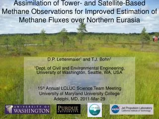
Estimating Soil Moisture, Inundation, and Carbon Emissions from Siberian Wetlands using Models and Remote Sensing T.J. Bohn1, E. Podest2, K.C. McDonald2, L. C. Bowling3, and D.P. Lettenmaier1 1Dept. of Civil and Environmental Engineering, University of Washington, Seattle, WA, USA 2JPL-NASA, Pasadena, CA, USA, 3Purdue University, West Lafayette, IN, USA NEESPI Workshop CITES-2009 Krasnoyarsk, Russia, 2009-July-14
Western Siberian Wetlands Wetlands: Largest natural global source of CH4 West Siberian Lowlands 30% of world’s wetlands are in N. Eurasia High latitudes experiencing pronounced climate change Response to future climate change uncertain (Gorham, 1991)
Climate Factors Temperature (via metabolic rates) CO2 CH4 CO2 Relationships non-linear Water table depth not uniform across landscape - heterogeneous NPP Living Biomass Acrotelm Temperature (via evaporation) Aerobic Rh Water Table Precipitation Anaerobic Rh Catotelm Note: currently not considering export of DOC from soils
Soil Surface Water Table Soil Surface Soil Surface Soil Surface Water Table Soil Surface Water Table Water Table Water Table Water Table Heterogeneity • Many studies assume uniform water table distribution within static, prescribed wetland area • Can lead to “binary” CO2/CH4 partitioning • Distributed water table allows smoother transition and more realistic inundated area • Facilitates comparisons with: • remote sensing • point observations Uniform Water Table Distributed Water Table Inundated Area Complete inundation No inundation
Questions How does taking water table heterogeneity into account affect: • comparisons of inundated area with remote sensing observations? • estimates of greenhouse gas emissions?
Modeling Framework • VIC hydrology model • Large, “flat” grid cells (e.g. 100x100 km) • On hourly time step, simulate: • Soil T profile • Water table depth ZWT • NPP • Soil Respiration • Other hydrologic variables… How to represent spatial heterogeneity of water table depth?
Spatial Heterogeneity of Water Table: TOPMODEL* Concept Pixel Count Soil surface Zwtmean (from VIC) Water Table Depth Zwti κmean Pixel Count Wetness index κi Relate distribution of water table to distribution of topography in the grid cell Start with DEM (e.g. SRTM3) • Essentially: • flat areas are wet (high κi ) • steep areas are dry (low κi ) For each DEM pixel in the grid cell, define topographic wetness indexκi = ln(αi/tanβi) αi = upslope contributing area tanβi = local slope Local water table depth Zwti = Zwtmean – m(κi- κmean) m = calibration parameter Wetness Index Distribution All pixels with same κ have same Zwt *Beven and Kirkby, 1979
Process Flow – VBM* * VIC-BETHY-Methane Using Farquhar C assimilation, dark respiration, etc. from BETHY (Knorr, 2000) Gridded Meteorological Forcings VIC Zwtmean Soil T profile NPP Topography(x,y) (SRTM3 DEM) TOPMODEL relationship Wetness index κ(x,y) for all grid cell’s pixels Zwt(x,y) Methane Emission Model (Walter and Heimann 2000) CH4(x,y) = f(Zwt(x,y),SoilT,NPP)
Close correspondence between: • wetness index distribution and • observed inundation of wetlands from satellite observations Study Domain: W. Siberia Wetness Index from GTOPO-30 and SRTM3 Yenisei R. Ural Mtns Bad DEM Quality Ob’ R. Chaya/Bakchar/ Iksa Basin Vasuygan Wetlands
Comparison with PALSAR • Spatial distribution of inundation compares favorably with remote sensing • This offers a method to calibrate model soil parameters Simulated Inundated Fraction (at optimal Zwt) Simulated Inundated Fraction (at optimal Zwt) Observed Inundated Fraction (PALSAR Classification) Observed Inundated Fraction (PALSAR Classification) ROI 3 2006-05-28 ROI 1 2006-06-09 ROI 2 2007-07-06 ROI 4 2007-07-18 Approx. 30 km
How do resulting emissions differ between uniform water table and distributed water table? Experiment: • Calibrate methane model to match in situ emissions at a point (Bakchar site, Friborg et al, 2003) • Distributed case: calibrate distributed model water table depth to match observed inundation CH4 • Uniform case: select water table timeseries from single point in the landscape having same long-term average methane emissions as the entire grid cell in the distributed case; apply this water table to entire grid cell Water Table Inundated Area (matching remote sensing)
Interannual Variability, 1948-2007 Possible trend in temperature, also in CH4 Uniform Water Table: Shallower than average of distributed case But never reaches surface; no inundation Resulting CH4 has higher variability than for distributed case Distributed case is buffered by high- and low-emitting regions Impact on trends? Distrib Water Table Uniform Water Table
Net Greenhouse Warming Potential • CH4 makes up small part of C budget, but large contribution to greenhouse warming potential • On 100-year timescale, GHWP(CH4) = approx. 23 * GHWP(CO2) NPP and RhCO2 approximately cancel Net GHWP essentially follows GHWP(CH4) • Uniform water table: • CH4 has larger interannual variability • So does net GHWP • Impact on trend assessment? NPP RhCO2 - NPP RhCO2 NET GHWP RhCH4
Interannual Variability, 1948-2007 How do spatial distributions of inundation and CH4 emissions change in response to climate? Example Years to investigate: 1980: “average” 1994: warm, dry 2002: warm, wet Distrib Water Table Uniform Water Table
Response to Climate 1980 = “average” year, in terms of T and Precip • 1994 = Warm, dry year • Less inundation • 2002 = Warm, wet year • More inundation • Increase in Tsoil increases CH4 emissions in wettest areas only • Increase in saturated area causes widespread increase in CH4 emissions
Conclusions • Advantages of distributed water table: • Facilitates comparison with satellite measurements and point measurements • More realistic representation of hydrologic and carbon processes • Spatial distribution of water table has large effect on estimates of greenhouse gas emissions and their trends
Thank You This work was carried out at the University of Washington and the Jet Propulsion Laboratory under contract from the National Aeronautics and Space Administration. This work was funded by NASA grant NNX08AH97G.
Calibration – Bakchar Bog, 1999 Soil T ZWT (water table depth) CH4 VBM = VIC-BETHY-Methane (Bohn et al., 2007)