Download
1 / 19
190 likes | 379 Views
Human Reward / Stimulus/ Response Signal Experiment: Data and Analysis. Draws on: Alan and Bill’s experiment Usher & McClelland model and experiments Patrick Simen’s model Sam and Phil’s analysis Juan’s further analysis.

E N D
Human Reward / Stimulus/ Response Signal Experiment: Data and Analysis Draws on: Alan and Bill’s experimentUsher & McClelland model and experimentsPatrick Simen’s model Sam and Phil’s analysis Juan’s further analysis
Human experiment examining reward bias effect with responsesignal given at different times after target onset • Target stimuli are rectangles shifted 1,3, or 5 pixels L or R of fixation • Reward cue occurs 750 msec before stimulus. • Small arrow head pointing L or R visible for 250 msec. • Only biased reward conditions (2 vs 1 and 1 vs 2) are used. • Response signal occurs at different times after target onset: 0 75 150 225 300 450 600 900 1200 2000 • Participant receives reward only if response is correct and occurs within 250 msec of response signal. • Participants were run for 15-25 sessions to provide stable data. • Data shown are from later sessions in which effects were all stable.
A participant with very little reward bias • Top panel shows probability of response giving larger reward as a function of actual response time for combinations of: Stimulus shift (1 3 5) pixels Reward-stimulus compatibility • Lower panel shows data transformed to z scores, and corresponds to the theoretical construct: mean(x1(t)-x2(t))+bias(t) sd(x1(t)-x2(t)) where x1 represents the state of the accumulator associated with greater reward, x2 the same for lesser reward,and S is thought to choose larger reward if x1(t)-x2(t)+bias(t) > 0.
Analysis Assumptions 0.6 -x • Decision variable x varies as a function of t. • Choice is made at some time t = signal lag + rt. • At the time the choice is made: • For a single difficulty level, two distributions, with means +m, -m, and equal sd s set to 1. Choose high reward if decision variable x > -Xc • For three difficulty levels, fixed s = 1, means mi (i=1,2,3),assume same Xc for all difficulty levels. • Xc can be regarded as a positive increment to the state of the decision variable;high reward is chosen if x > 0 in this case. 0.5 c m m + - 0.4 0.3 0.2 0.1 0 -10 -8 -6 -4 -2 0 2 4 6 8 10
Only one diff level Three diff levels Subject’s sensitivity, as defined in theory of signal detectability When response signal delay varies For each subject, fit with function from UM’01
Observed “bias”, treatedas positive offsetfavoring response associated with highreward. 1.5 -Xc/s 1 Optimal “bias” Xc/sbased on observedsensitivity data. 0.5 0 -10 -8 -6 -4 -2 0 2 4 6 8 10
Some possible models • OU process (l < 0, n0 = 0) following F&H,with reward bias effect implemented as: • An alteration in initial condition, subject to decay • Optimal time-varying decision boundary outside of the OU process • An input ‘current’ starting at presentation of reward signal • Noise from reward onset • Noise from stimulus onset • A constant offset or criterion shift unaffected by time
1. Reward as a change in initial condition, subject to decay • Note: • Effect of the bias decays away for lambda<0. • There is a dip at • At t=0, p=1. Feng & Holmes notes
2. Time-varying optimal bias (Outside of OU process) • Note: • Effect of the bias persists. • There is a dip at • At t=0, p=1. • The smaller the stimulus effect, the larger the bias. • The harder the stimulus condition, the later the dip.
3.1. Reward acts as input “current”, stays on from reward signal to end of trial, noise starts at reward onset Reward signal comes t seconds before stimulus 2l • Note: • Effect of the bias persists • There is no dip. • At t=0, p<1. Feng & Holmes notes
3.2. Same as 3.1 but variability is introduced only at stimulus onset 2l • Note: • Effect of the bias persists • There is dip at • At t=0, p=1 since all accumulators have no variance.
4. Reward as a constant offset • Note: • Equivalent to 3.2for large lt • There is a dip at • At t=0, p=1
Some possible models • OU models (l < 0, n0 = 0) following F&H,with reward bias effect implemented as: • An alteration in initial condition, subject to decay • Optimal time-varying decision boundary outside of the OU process • An input ‘current’ starting at presentation of reward signal • Noise from reward onset • Noise from stimulus onset • A constant offset or criterion shift unaffected by time • While none fit perfectly, starting point variability (n0 > 0) would potentially improve 3.2 and 4.
Jay’s favorite mechanistic story(draws from Simen’s model) • Participant learns to inject waves of activation that prime response accumulators; waves peak just after stimulus onset and have a residual. • Wave is higher for hi rwd response. • Stimulus activation accumulates as in LCAM. • Response signal initiates added drive to both accumulators equally. • First accumulator to fixed threshold initiates the response.