Performance Modelling in Queue Networks for Efficient Resource Management
Learn about Mean Value Analysis (MVA) for open and closed queue networks to optimize performance. Understand outgoing and incoming request handling, CPU, disk, tape resources, and more. Improve resource utilization efficiency.

Performance Modelling in Queue Networks for Efficient Resource Management
E N D
Presentation Transcript
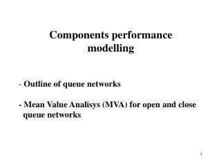
Components performance modelling • Outline of queue networks- Mean Value Analisys (MVA) for open and close • queue networks
outgoing requests incoming requests CPU DISK DISK TAPE TAPE M clients CPU Open queue network Closed queue network (number finite of users)
Kind of resources in a queue network S(n) R(n) Load independent n S(n) R(n) Load dependent n S(n) R(n) Delay n
Definitions K: number of queues X0: network average throughput. If open network in a stationary condition X0 = Vi: average number of visits a generic request makes to i server from its generation to its service time (request goes out from the system if open network) Si: average request service time at the server i Wi: average request waiting time in the queue i Ri: average request answer time in the queue i Ri = Si + Wi
Definitions Xi: throughput for the i-th queue Xi =X0 Vi R’i: average request residence time in the queue i from its creation to its service time (request goes out from the system if open network) R’i =Vi Ri Di: request service demand to a server in a queue i from its creation to its service time (request goes out from the system if open network) Di =Vi Si
Qi: total time a request spends waiting in the queue i from its creation to its service time (request goes out from the system if open network) Qi =Vi Wi ------------------------------- R’i =Vi Ri =Vi (Wi +Si) =Wi Vi + Si Vi = Qi +Di ------------------------------- R0: average request answer time from the whole system R0 = ki=1 R’i ni: average number of requests waiting or in service at the queue i N: average number of requests in the system N = ki=1 ni
Open queue network outgoing requests incoming requests CPU DISK TAPE 7
Open networks (Single Class) Equations: Arrival theorem (for open networks): the average number of requests in a queue i that an incoming request find in the same queue (nai), is equal to the average number of requests in the queue i (ni). Ri(n) = Si + Wi(n) = Si + ni Si Using Little’s Law (ni = Xi Ri) and Ui = XiSi: Ri = Si _ (1-Ui) Ri = Si (1 + ni) = Si + Si Xi Ri Ri (1- Ui) = Si
Open networks (Single Class) Equations: Then: . R’i = Vi Ri = Di _ (1-Ui) Besides: . ni = Ui _ (1-Ui) Because Ui = Xi Si
Open networks(Single Class) Calculation of the greatest : In an open network the average frequency of users incoming into the network is fixed. For too much big the network will become unstable, we are then interested in the greatest value of that we can apply to the network. Because: Ui = Xi Si = Vi Si then: = Ui / Di because Di = Vi Si Ui = 1 for the greatest use of the queue i, then we can calculate the greatest that doesn’t make unstable the system: 1 _ maxki=1 Di
DISK2 DISK1 CPU DB Server(example 1) 10.800 request per hour = X0 DCPU = 0,2 sec Service demand at CPU VDISK1 = 5 VDISK2 = 3 SDISK1 = SDISK2 = 15 msec DDISK1 = VDISK1 * SDISK1 = 5 * 15 msec = 75 msec Service demand at disk 1 DDISK2 = VDISK2 * SDISK2 = 3 * 15 msec = 45 msec Service demand at disk 2
DISK2 DISK1 CPU DB Server(example 1) . Service Demand Law UCPU = DCPU * X0 = 0,2 sec/req * 3 req/sec = 0,6 CPU utilization UD1 = DDISK1 * X0 = = 0,225 Disk1 utilization UD2 = = 0,135 Disk2 utilization Residence time R’CPU = DCPU / (1- UCPU ) = 0,5 sec R’D1 = DDISK1 / (1- UDISK1 ) = 0,097 sec R’D2 = DDISK2 / (1- UDISK2 ) = 0,052 sec
Total response time R0 = R’CPU + R’D1 + R’D2 = 0,649 sec Average number of requests at each queue nCPU = UCPU / (1- UCPU ) = 0,6 / (1-0,6) = 1,5 nDISK1 = = 0,29 nDISK2 = = 0,16 Total number of requests at the server N = nCPU + nDISK2 +nDISK2 = 1,95 requests RMaximum arrival rate = 1 _ = 1 _ = 5 req /sec maxki=1 Di max (0,2; 0,075; 0,045)
DISK TAPE M clients CPU Closed queue network (number finite of users) 14
Closed networks(Mean Value Analysis) • Allows calculating the performance indexes (average response time, throughput, average queue lenght, etc…) for a closed network • Iterative method based on the consideration that a queue network results can be calculated from the same network results with a population reduced by one unit. • Useful also for hybrid queue networks Definitions .X0: average queue network throughput. . Vi: average number of visits for a request at a queue i. . Si: average service time for a request on the server i. . Ri: average stay time for a request at the queue i.
Closed networks(Mean Value Analysis) Definitions . R’i: total average stay time for a request at the queue i considering all its visits at the queue. Equal to Vi Ri . Di: total average service time for a request at the queue i considering all its visits at the queue. Equal to Vi Si . R0: average response time of the queue network. Equal to the sum of theR’i . nia: average number of the requests found by a request incoming in the queue. Forced Flow Law Then we have: . Xi = X0 Vi
Mean Value Analysis (Single class) Equations: Ri(n) = Si + Wi(n) = Si + nia(n) Si = Si (1+ nia(n) ) Arrival Theorem: the average number of requests (nia) in a queue i thatan incoming request find in the same queue, is equal to the average number of requests in the queue i if n-1 requests are in the queue network (ni(n-1) that is n minus what wants the service on the i-th queue) in other words: nia(n) = ni(n-1) then: Ri = Si(1+ni(n-1)) and multiplying both members for Vi →R’i = Di(1+ni(n-1))
Mean Value Analysis (Single class) Equations: Applying Little’s Law to the whole “queue network” system (n=X0R0), we have: →X0 = n / R0(n) = n / Kr=1 R’i(n) Applying Little’s Law and Forced Flow Law: → ni(n) = Xi(n) Ri(n) = X0(n) Vi Ri(n) = X0(n) R’i(n)
Mean Value Analysis (Single class) Three equations: →Residence Time equation R’i = Di[1+ni(n-1)] →Throughput equation X0 = n / Kr=1 R’i(n) →Queue lenght equation ni(n) = X0(n) R’i(n) 19
Mean Value Analysis (Single class) Iterative procedure: • We know that ni(n) = 0 for n=0: if no message is in the queue network, then no message will be in every single queue. • Given ni(0) it’s possible to evaluate all R’i(1) • Given all R’i(1) it’s possible to evaluate all ni(1) and X0(1) • Given all ni(1) it’s possible to evaluate all R’i(2) • The procedure continues until all ni(n), R’i(n) and X0(n) are found, where n is the number of requests inside the network.
DB Server(example 2) • Requests from 50 clients • Every request needs 5 record read from (visit to) a disk • Average read time for a record (visit) = 9 msec • Every request to DB needs 15 msec CPU DCPU = SCPU = 15 msecCPU service demand DDISK = SDISK * VDISK = 9 * 5 = 45 msecDisk service demand
DB Server(example 2) UsingMVA Equations n = 0; Number of concurrent requests R’CPU = 0; Residence time for CPU R’DISK = 0; Residence time for disk R0 = 0; Average response time X0 = 0; Throughput nCPU = 0; Queue lenght at CPU nDISK = 0 Queue lenght at disk n = 1; R’CPU = DCPU (1+ nCPU(0)) = DCPU = 15 msec; R’DISK = DDISK (1+ nDISK(0)) = DDISK = 45 msec; R0 = R’CPU + R’DISK = 60 msec; X0 = n/ R0 = 0,0167 tx/msec nCPU = X0 * R’CPU = 0,250 nDISK = 0,750
DB Server(example 2) n = 1; R’CPU = DCPU (1+ nCPU(0)) = DCPU = 15 msec; R’DISK = DDISK (1+ nDISK(0)) = DDISK = 45 msec; R0 = R’CPU + R’DISK = 60 msec; X0 = 1 / R0 = 0,0167 tx/msec nCPU = X0 * R’CPU = 0,250 nDISK = 0,750 n = 2; R’CPU = DCPU (1 + nCPU(1)) = 15 * 1,25 = 18,75 msec; R’DISK = DDISK (1 + nDISK(1)) = 45 * 1,750 = 78,75 msec; R0 = R’CPU + R’DISK = 97,5 msec; X0 = 2 / R0 = 0,0333 tx/msec nCPU = X0 * R’CPU = 0,625 nDISK = X0 * R’DISK = 2,625 23
Closed networks (Single Class) - Bounds Bottleneck identification (1/3) Usually the queue network throughput will reach saturation if requests increase inside the system; we are then interested in finding the component in the system that causes saturation. → in open networks: 1 _ maxki=1 Di and replacing with X0 (n): X0 (n) 1 _ maxki=1 Di
Closed networks (Single Class) - Bounds Bottleneck identification (2/3) • from throughput equation of MVA, remembering that R’i (n)= Di [1 + ni(n)] → R’i Di for every queue i, then we have: X0 (n) = nn _ Kr=1R’iKr=1Di
X0 n Closed networks (Single Class) - Bounds Bottleneck identification (3/3) • Combining the preceding two equations we obtain: → X0 (n) min n _ , 1 _ Kr=1Di maxki=1 Di For little n the throughput will increase at the most in a linear way with n, then becomes flat around the value 1/maxki=1 Di
Closed networks (Single Class) - Bounds Average response time (1/2) When throughput reaches its greatest value (that is for n big) the average response time is equivalent to: R0 (n) n _ max throughput Then for n big the response time increases in a linear way with n: → R0 (n) n maxki=1 Di On the contrary, for small values of n (n near to 1) the average response time will be: → R0 (n) = Kr=1Di considering that all waiting times are null.
Closed networks (Single Class) - Bounds Average response time (2/2) We can establish a lower bound on average response time equal to: → R0(n) max Ki=1Di , n ∙maxki=1 Di
DB Server(Example 3) New scenarios with regard to preceding example: • index variation in DB (# of disk access equal to 2,5 (before was 5)) • 60% faster Disk (average service time = 5,63 msec) • faster CPU (service demand = 7,5 msec)