Download
1 / 53
530 likes | 657 Views
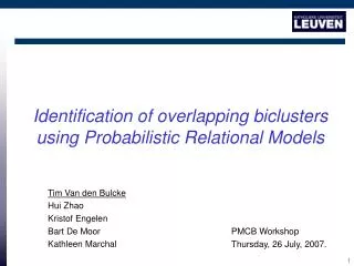
Identification of overlapping biclusters using Probabilistic Relational Models. Tim Van den Bulcke, Hui Zhao , Kristof Engelen, Bart De Moor, Kathleen Marchal. Overview. Biclustering and biology Probabilistic Relational Models Pro Bic biclustering model Algorithm Results Conclusion.

E N D
Identification of overlapping biclusters using Probabilistic Relational Models Tim Van den Bulcke, Hui Zhao, Kristof Engelen, Bart De Moor, Kathleen Marchal
Overview • Biclustering and biology • Probabilistic Relational Models • ProBic biclustering model • Algorithm • Results • Conclusion
Overview • Biclustering and biology • What is biclustering? • Why biclustering? • Probabilistic Relational Models • ProBic biclustering model • Algorithm • Results • Conclusion
Biclustering and biology What is biclustering? • Definition in the context of gene expression data: A biclusteris a subset of genes which show a similar expression profile under a subset of conditions. conditions genes
Biclustering and biology Why bi-clustering?* • Only a small set of the genes participates in a cellular process. • A cellular process is active only in a subset of the conditions. • A single gene may participate in multiple pathways that may or may not be coactive under all conditions. * From: Madeira et al. (2004) Biclustering Algorithms for Biological Data Analysis: A Survey
Overview • Biclustering and biology • Probabilistic Relational Models • ProBic biclustering model • Algorithm • Results • Conclusion
Probabilistic Relational Models (PRMs) Contact Virus strain Patient Treatment Image: free interpretation from Segal et al. Rich probabilistic models
Probabilistic Relational Models (PRMs) • Traditional approaches “flatten” relational data • Causes bias • Centered around one view of the data • Loose relational structure • PRM models • Extension of Bayesian networks • Combine advantages of probabilistic reasoning with relational logic Contact Patient flatten
Overview • Biclustering and biology • Probabilistic Relational Models • ProBic biclustering model • Algorithm • Results • Conclusion
ProBic biclustering model: notation • g: gene • c: condition • e: expression • g.Bk: gene-bicluster assignment for gene g to bicluster k (unknown, 0 or 1) • c.Bk: condition-bicluster assignment for condition c to bicluster k (unknown, 0 or 1) • e.Level: expression level value (known, continuous value)
ProBic biclustering model • Dataset instance Gene Condition Expression
P(e.level | g.B1,g.B2,c.B1,c.B2,c.ID) = Normal( μg.B,c.B,c.ID, σg.B,c.B,c.ID ) 1 2 3 ProBic biclustering model • Relational schema and PRM model Notation: • g: gene • c: condition • e: expression • g.Bk: gene-bicluster assignment for gene g to bicluster k (0 or 1, unknown) • c.Bk: condition-bicluster assignment for condition c to bicluster k: (0 or 1, unknown) • e.Level: expression level value (continuous, known) Gene Condition ID B1 B2 B1 B2 Expression level P(e.level | g.B1,g.B2,c.B1,c.B2,c.ID) = Normal( μg.B,c.B,c.ID, σg.B,c.B,c.ID )
Gene Condition Gene Condition ID B1 B2 ID ID B1 B2 B1 B2 B1 B2 g1 ? (0 or 1) ? (0 or 1) c1 ? (0 or 1) ? (0 or 1) g2 ? (0 or 1) ? (0 or 1) c2 ? (0 or 1) ? (0 or 1) c2.B1 c2.B2 c1.B1 c1.B2 Expression Expression level g.ID c.ID level c2.ID g1 c1 -2.4 c1.ID g1 c2 (missing value) g2 c1 1.6 P(e.level | g.B1,g.B2,c.B1,c.B2, c.ID) = Normal( μg.B,c.B, c.ID, σg.B,c.B,c.ID ) g1.B2 g2 c2 0.5 g1.B1 level1,1 g2.B2 g2.B1 level2,1 level2,2 ProBic biclustering model PRM model Database instance ground Bayesian network
Expression level prior (μ, σ)’s Expression level conditional probabilities Prior gene to bicluster assignment Prior condition to bicluster assignments ProBic biclustering model • Joint Probability Distribution is defined as a product over each of the node in Bayesian Network: • ProBic posterior ( ~ likelihood x prior ):
Overview • Biclustering and biology • Probabilistic Relational Models • ProBic biclustering model • Algorithm • Results • Conclusion
Algorithm: choices • Different approaches possible • Only approximative algorithms are tractable: • MCMC methods (e.g. Gibbs sampling) • Expectation-Maximization (soft, hard assignment) • Variational approaches • simulated annealing, genetic algorithms, … • We chose a hard assignment Expectation-Maximization algorithm (E.-M.) • Natural decomposition of the model in E.-M. steps • Efficient • Extensible • Relatively good convergence properties for this model
Algorithm: Expectation-Maximization • Maximization step: • Maximize posterior w.r.t. μ, σ values (model parameters), given the current gene-bicluster and condition-bicluster assignments (=the hidden variables) • Expectation step: • Maximize posterior w.r.t. gene-bicluster and condition-bicluster assignments, given the current model parameters • Two-step approach: • Step 1: max. posterior w.r.t. C.B, given G.B and μ, σ values • Step 2: max. posterior w.r.t. G.B, given C.B and μ, σ values
Overview • Biclustering and biology • Probabilistic Relational Models • ProBic biclustering model • Algorithm • Results • Noise sensitivity • Bicluster shape • Overlap • Missing values • Conclusion
Results: noise sensitivity • Setup: • Simulated dataset: 500 genes x 200 conditions • Background distribution: Normal(0,1) • Bicluster distributions: Normal( rnd(N(0,1)), σ ), varying sigma • Shapes: three 50x50 biclusters
A … B … A B A B Results: noise sensitivity Recall (genes) Precision (genes) A B σ σ Precision (conditions) Recall (conditions) B A σ σ Precision = TP / (TP+FP) Recall = TP / (TP+FN)
Results: bicluster shape independence • Setup: • Dataset: 500 genes x 200 conditions • Background distribution: N(0,1) • Bicluster distributions: N( rnd(N(0,1)), 0.2 ) • Shapes: 80x10, 10x80, 20x20
Results: Overlap examples • Two biclusters (50 genes, 50 conditions) • Overlap:25 genes, 25 conditions • Two biclusters (10 genes, 80 conditions) • Overlap: 2 genes, 40 conditions
Results: Missing values • ProBic model has no concept of ‘missing values’ No prior missing value estimations which could bias the result
Results: Missing values – one example • 500 genes x 200 conditions • Noise std: bicluster 0.2, background 1.0 • Missing value: 70% • One bicluster 50x50
Results: Missing values Recall (genes) Precision (genes) % missing values Precision (conditions) Recall (conditions) % missing values
Overview • Biclustering and biology • Probabilistic Relational Models • ProBic biclustering model • Algorithm • Results • Conclusion
Conclusion • Noise robustness • Naturally deals with missing values • Relatively independent of bicluster shape • Simultaneous identification of multiple overlapping biclusters • Can be used query-driven • Extensible
Acknowledgements KULeuven: • whole BioI group, ESAT-SCD • Tim Van den Bulcke • Thomas Dhollander • whole CMPG group(Centre of Microbial and Plant Genetics) • Kristof Engelen • Kathleen Marchal UGent: • whole Bioinformatics & Evolutionary Genomics group • Tom Michoel
Promoter S1 S2 S3 S4 Gene R1 R2 R3 Array M1 M2 P1 P2 P3 M1 M2 Expression level Near future • Automated definition of algorithm parameter settings • Application biological datasets • Dataset normalization • Extend model with different overlap models • Model extension from biclusters to regulatory modulesinclude motif + ChIP-chip data R1 R2 ACAGG TTCAAT …
Gene Condition ID B1 B2 B1 B2 c2.B1 c2.B2 c1.B1 c1.B2 ID B1 B2 ID B1 B2 g1 ? (0 or 1) ? (0 or 1) Expression c1 ? (0 or 1) ? (0 or 1) g2 ? (0 or 1) ? (0 or 1) c2 ? (0 or 1) ? (0 or 1) level c2.ID c1.ID g1.B2 P(e.level | g.B1,g.B2,c.B1,c.B2, c.ID) = Normal( μg.B,c.B, c.ID, σg.B,c.B,c.ID ) g.ID c.ID level g1.B1 level1,1 g1 c1 -2.4 g1 c2 (missing value) g2 c1 1.6 g2 c2 0.5 g2.B2 level2,2 g2.B1 level2,1 Results: Missing values • ProBic model has no concept of ‘missing values’ PRM model Database instance Condition Gene Expression ground Bayesian network
Algorithm properties • Speed: • 500 genes, 200 conditions, 2 biclusters: 2 min. • Scaling: • ~ #genes . #conditions . 2#biclusters (worse case) • ~ #genes . #conditions . (#biclusters)p (in practice), p=1..3
Overview • Biclustering and biology • Probabilistic Relational Models • ProBic biclustering model • Algorithm • Results • Discussion • Conclusion
Discussion: Expectation-Maximization • Initialization: • initialization with (almost) all genes and condition: convergence to good local optimum • multiple random initializations: many initializations required (speed!) • E.-M. steps: • limit changes in gene/condition-bicluster assignments in both E-steps results in higher stability (at cost of slower convergence)
Objects Attributes Probabilistic Relational Models (PRMs) • Relational extension to Bayesian Networks (BNs): • BNs ~ a single flat table • PRMs ~ relational data structure • A relational scheme (implicitly) defines a constrained Bayesian network • In PRMs, probability distributions are shared among all objects of the same class • Likelihood function:(very similar to chain-rule in Bayesian networks) • Learning PRM model e.g. using maximum likelihood principle
Algorithm: user-defined parameters • P(μg.B,c.B,c, σg.B,c.B,c): prior distributions for μ, σ • Conjugate: • Normal-Inverse-χ2 distribution or • Normal distribution with pseudocount • Makes extreme distributions less likely • P(a.Bk): prior probability that a condition is in bicluster k • Prevents background conditions to be in biclusters • If no prior distribution P(μ, σ): conditions are always more likely to be in a bicluster due to statistical variations. • P(g.Bk): prior probability that a gene is in bicluster k • Initialize biclusters with seed genes: query-driven biclustering • P(a.Bk) andP(g.Bk): • Both have impact on the preference for certain bicluster shapes
Algorithm: Expectation-Maximization • Expectation step 2: • argmaxG.Blog(posterior) constant without prior: independent per gene Approximation based on previous iteration quasi independence if small changes in assignment
ProBic biclustering model 1 PRM model Gene Condition ID B1 B2 B1 B2 Expression level 2 c=44 P(e.level | g.B1,g.B2,c.B1,c.B2, c.ID) = Normal( μg.B,c.B, c.ID, σg.B,c.B,c.ID )
ProBic biclustering model • ground Bayesian network c2.B1 c2.B2 c1.B1 c1.B2 c2.ID c1.ID g1.B2 g1.B1 level1,1 g2.B2 g2.B1 level2,1 level2,2
Objects Attributes ProBic biclustering model • Likelihood function:(~ chain-rule in Bayesian networks) • In PRMs, probability distributions are shared among all objects of the same class
constant independent per condition + analytic solution based on sufficient statistics Algorithm: Expectation-Maximization • Maximization step: • argmaxμ,σlog(posterior)
constant independent per condition Algorithm: Expectation-Maximization • Expectation step 1: assign conditions • argmaxC.Blog(posterior)
c.B = 1 ? c.B = 1,2 ? c.B = 1,2,3 ? Algorithm: Expectation-Maximization • Expectation step 1: • Evaluate function for every condition and for every bicluster assignment e.g. 200 conditions, 30 biclusters: 200 * 230 = 200 billion~ a lot • But can be performed very efficiently: • Partial solutions can be reused among different bicluster assignments 1 2 3
a.B = 1 ? a.B = 2 ? a.B = 1,2 ? Algorithm: Expectation-Maximization • Expectation step 1: • Evaluate function for every condition and for every bicluster assignment e.g. 200 conditions, 30 biclusters: 200 * 230 = 200 billion~ a lot • But can be performed very efficiently: • Partial solutions can be reused among different bicluster assignments • Only evaluate potential good solutions: use Apriori-like approach. 1 2 3
Algorithm: Expectation-Maximization • Expectation step 1: • Evaluate function for every condition and for every bicluster assignment e.g. 200 conditions, 30 biclusters: 200 * 230 = 200 billion~ a lot • But can be performed very efficiently: • Partial solutions can be reused among different bicluster assignments • Only evaluate potential good solutions: use Apriori-like approach. • Avoid background evaluations 1 2 3
Algorithm: Expectation-Maximization • Expectation step 2: • Analogous approach as in step 1
. . B O I I Acknowledgements KULeuven: • whole BioI group, ESAT-SCD • Tim Van den Bulcke • Thomas Dhollander • whole CMPG group(Centre of Microbial and Plant Genetics) • Kristof Engelen • Kathleen Marchal UGent: • whole Bioinformatics & Evolutionary Genomics group • Tom Michoel