Download
1 / 44
450 likes | 637 Views
ESS 261 Spring Quarter 2009. Waves and Discontinuities Fourier Series and Wavelet Analysis Wave Polarization, Ellipticity Minimum Variance Analysis Rankine-Hygoniot Relations, Coplanarity Shock Normal, Shock Propagation Speed Contributions from K. K. Khurana, R. W. Walker

E N D
ESS 261 Spring Quarter 2009 Waves and Discontinuities Fourier Series and Wavelet Analysis Wave Polarization, Ellipticity Minimum Variance Analysis Rankine-Hygoniot Relations, Coplanarity Shock Normal, Shock Propagation Speed Contributions from K. K. Khurana, R. W. Walker References: ISSI book on Analysis Methods for Multi-Spacecraft Data Lecture 05 April 27, 2009 1
Fourier Series • Any periodic function (a(t+T)=a(t)) where w=2p/T is the frequency can be expressed as a Fourier series • a(t) must satisfy the condition • Any “reasonable” function satisfying the above condition can be expanded as a function of sin and cos • To find the coefficients use the following relationships which result because sin and cos are an “orthogonal” basis of functions. 2
Fourier Series in Complex Form • The Fourier expansion can be generalized for complex variables if the basis functions are allowed to include complex components. Using the basis functions: cos(nt)i sin(n t)=e-( it) and complex amplitudes, it is possible to decompose arbitrary real and imaginary functions as: • Negative frequencies represent same time-scale oscillations as positive frequencies; by adding or subtracting them one can obtain only real or only imaginary signals. E.g., • For a real signal: • You can show easily that: • And for real signals: • This is Parseval’s Theorem and states that the average energy in the signal, i.e., the signal power, is the sum of the power contribution from each frequency component. 3
Power Spectral Density • If the expanded interval is twice as long, 2T, the number of frequency bins below a given max. frequency maxdoubles: n’* ’ =n’*(2/T’)=n’*(2/(2T))=(n’/2)*(2/T)< max therefore n’=2n, where n’ is the new cutoff harmonic in the expansion. This is because the minimum discrete frequency step (frequency unit) depends on the total length of the interval being expanded f=1/T and == 2/T. • As the number of Fourier components increases the amplitude of each has to decrease proportionately, to preserve the same total power. The amplitudes in the right hand of depend on the signal length, which is not really appealing. • The power spectral density (PSD) is defined as power per unit frequency bin, and avoids dependence on signal length: • The PSD is defined only for real signals. Parseval’s theorem becomes a sum of power spectral densities independent of signal length, which is a continuous function of frequency as the time series becomes infinite. 4
Discrete Fourier Transform (DFT) • Assuming discrete time series, of finite number of points, N, equally spaced by t=T/N , the time series is: a(tj)=a(t0+j*t), j=0,1,…N-1. Then by approximating the integral in the Fourier amplitude with a sum, we obtain the Discrete Fourier Transform equations: • For real signals, negative components carry no new information, as: • Shifting the sum over Fourier space, n, by N results in no difference in the outcome • The inverse transform is often expressed as: • The Parseval Theorem becomes: • Since there is no new information beyond term N/2, fNyquist=1/2t defines the max freq. of interest 5
DFT: Normalization can be tricky and confusing (ISSI SR-001) 6 From: ISSI Sci. Rep. SR-001 (Analysis Methods fo Multi-Spacecraft Data)
Some Useful Properties of Fourier Series • Periodicity – Fourier series are periodic with defined period. The Fourier series converges on the required function only in the given interval. • Even and odd functions - The sine is odd (a(-t)=-a(t)) while cosine is even (a(-t)=a(t)). Fit even functions with cosine and odd function with sine. • Half-period series – A function a(t) defined only on the interval (0,T) can be fit with either sines or cosines. • Least squares approximation- When a Fourier series expansion of a continuous function a(t) is truncated after N terms it is a least squares fit to the original. The area of the squared difference between the two functions is minimised and goes to zero as N increases. • Gibbs phenomenon- The Fourier series converges in the least-squares sense when a(t) is discontinuous but the truncated series oscillates near the discontinuity. 7
The Fourier Integral • The Fourier integral transform (FIT) F(w) of a function f(t) is defined as • The inverse transform is • The right hand side is finite if 8
The Fourier Integral Transform Continued • The condition is very restrictive. It means that simple functions like f(t)=const. or sin wt won’t work. • This can be fixed by using the Dirac delta function d(t) (d(t)=0, t≠0; ) • The substitution property makes integration trivial • Apply the definition of the FIT to the delta function • .This gives • Apply the definition of the FIT to the delta function in fourier space: • For monchromatic waves 9
The z-Transform • Assume we have series of measurements spaced evenly in time (or space) {a}= a0,a1,a2,…,aN-1 • A z-transform is made by creating a polynomial in the complex variable z using • Operations on the z –transform all have counterparts in the time domain. • Imagine multiplying the z-transform by z This new transform is what you would get if you shifted the original time series by one unit in time. In this case z is called the unit delay operator. • Multiplication of two z-transforms is called discrete convolution. The discrete convolution theorem is what gives the z-transform its power. 10
…continued • Consider the product of A(z) and B(z) each of different length. • Set p=k+l and change the order of summation • This is the z-transform of a time series of length N+M-1. • c=a*b is the “discrete convolution” of a, b • The discrete convolution theorem for z-transformations is given by the following notation: • Division by a z-transform is deconvolution. As long as a0≠0 then b0=c0/a0, b1=(c1-a1b0)/a0 and • This is a recursive procedure because the result of each equation is used in all subsequent equations. 11
The Discrete Fourier Transform revisited • Substitute z=e-iwDt into the z-transform equations and normalize by N • This equation is a complex Fourier series that is a continuous function of frequency that has been discretized so that where Δf is the sampling frequency. • The DFTis therefore a Z-transform using a basis function on unit circle • This formula transforms the N values of the time sequences {ak} into another sequence of numbers with N Fourier coefficients {Ak}. • The inverse equation to recover the original time series from the Fourier coefficients is: • k measures time in units of Δt up to a maximum of T=NΔt. n measures frequency intervals of Δν=1/T up to a maximum of vs=NΔν=1/ Δt . 12
Amplitude, Power and Phase Spectra • The Fourier coefficients An describe the contribution of the particular frequency w=2pnDn to the original time sequence. • A signal with just one frequency is a sine wave. • Rn is the maximum • Φn defines the initial point in the cycle. • Rn plotted against n is called the amplitude spectrum • Rn2 plotted against n is the power spectrum. • Φn is an angle that describes the phase of this frequency with the timeseries and the corresponding plot is a phase spectrum. • The Shift Theorem – multiplication of the DFT by e-iwDt will delay the sequence by one sampling interval. In other words shifting the time sequence one space will multiple the DFT coefficient An by e-2pin/N. The power spectrum is not changed but the phase is retarded by 2pn/N. • In deriving the convolution theorem we omitted terms in the sum involving elements of a or b with subscripts outside of the specified ranges, 0 to N-1 for a and 0 to M-1 for b. This is no longer correct for periodic functions. Practically this is made to work by padding with zeros to extend both series to length N+M+1. 13
Differentiation and Integration • Differentiation and integration only apply to continuous functions of time so we set t=kΔt and wn=2pn/NDt so the DFT becomes • Differentiating with respect to time gives • Make this discrete by setting t=kΔt and call so that • This is the inverse DFT so and iwnAnmust be transforms of each other. • Differentiation with respect to time is equivalent to multiplication by frequency in the frequency domain. • Integration with respect to time is equivalent to division in the frequency domain. 14
Aliasing and Shannon’s Sampling Theorem • The transformation pair and are exact. Before digitizing we had continuous functions of time. • The periodicity of the DFT gives AN+n=An. • If the data are real AN-n=An*. • These equations define aliasing which is the mapping of higher frequencies into the range 0 to N/2 – after digitization higher frequencies are mapped to lower frequencies. • Fourier coefficients for frequencies above N/2 are determined exactly from the first N/2+1. • Above N they are periodic and between N/2 and N reflect with the same amplitude and phase change of π. • The DFT allows us to transform N real values in the time domain into any number of complex values An. • The highest meaningful coefficient in the DFT is AN/2 and the corresponding frequency is the Nyquist frequency fN=1/2Dt. • We can recover the original signal from digitized samples provided the original sample contained no energy above the Nyquist frequency. • To reproduce the original time series a(t) from its samples ak=a(kDt) we can use Shannon's theorem, which states that if the signal contains no power above frequency N/2Hz, it can be reconstructed from N measurements. 15
The Fast Fourier Transform • The DFT requires a sum over N terms for each of N frequencies. Thus the total number of calculations required goes as N2. This was a major impediment to doing spectral analysis. • The fast Fourier transform (FFT) allowed this to be done much faster. • Suppose that N is divisible by 2. Split the DFT into two parts. • This sum requires us to form the quantity in () (N/2 calculations) and then doing this N/2 times. For all frequencies this means calculations or a reduction of a factor of 2 for large calculations. • This procedure can be repeated. As long as N is a power of 2 the sum can be divided log2N times, with a total of 4Nlog2N operations. 16
The Fourier Transform of a Box Car • The Discrete Fourier Transform of a box car has a central peak and oscillations in frequency. 17
Filtering: The Running Average • Filtering is convolution with a second- usually shorter- time series. • Bandpass filters (fmin-fmax) eliminate ranges of frequencies from the time series. • Low-pass filters eliminate all frequencies above a certain frequency. • High-pass filters eliminate all frequencies below a certain frequency. • The range of frequencies allowed is called the pass band =fmin-fmax. • The critical frequencies are called cut-off frequencies. • A running average in which each member of a time series is replaced by an average of M neighboring members is a filter. • It is a convolution of the original time sequence with a boxcar function. • Intuitively we would expect the running average to remove high frequencies and therefore be a low-pass filter. • Since convolution in the time domain is multiplication in the frequency domain we have multiplied the DFT of the time series with the Fourier transform of the boxcar. • This is not an ideal low-pass filter because of the side lobes and the central peak let through a lot of energy above the desired frequency. • The amplitude spectrum is exactly zero at the frequencies (nN/MT) where the box car transform is zero so this filter is great if you want to eliminate a given frequency. 18
Filtering: Other windows Hamming Triangular Gaussian 19
Filtering: Some Examples • An ideal low-pass filter should have an amplitude spectrum that is zero outside of the cut-off frequency and one inside it. Gibb's phenomenon prevents such a filter from doing a good job as a low-pass filter. • We need to taper the filter like we tapered the window. • One example is the Butterworth filter ( ) where wC is the cut-off frequency at which the energy is halved. n controls the sharpness of the cut-off (order of the filter, or pole). • The corresponding high-pass filter is . • A bandpass filter can be made by shifting the frequency along the frequency axis to center it around wb . • A notch filter can be made from . • To construct the time sequence specify the phase (usually zero) and take the inverse Fourier transform. 20
Butterworth filter response … compared to others 21
Tapering (windowing) • In an ideal universe data would be a continuous function of time going forever, then the Fourier integral transform would give the spectrum. • In reality data are limited and the finite length T limits the frequency spacing to • The sampling interval Dt limits the maximum meaningful frequency to fNyquist. • It is frequently useful to assume a finite time series is a section of an infinite series. This is called windowing and is achieved by multiplying the time series by a box car (called a taper) that is zero outside of the window and one inside. • Since multiplication in the time is the same as convolution in frequency domain, this is equivalent to convolution with the DFT of a box car • A single peak is spread across a range of frequencies. • This is called spectral leakage. • Comes from the jumps at the edges of the time series. • We can improve this by using a window with different side lobes. For resolving peaks we want a narrow function in the frequency domain but that means a broad function in the time domain – the uncertainty principle. • Time windowing can reduce noise by smoothing; the spectrum- noise reduction comes at the expense of time resolution • PSD must be normalized due to power loss from windowing. 22
Detrending and averaging • Signal is assumed infinite, periodic and thus continuous but in reality it is finite, aperiodic and discontinuous. Trends due to very low frequency signals (unresolved) will cause a jump at the edge, giving low frequency power that is unrealistic. Trend can be removed by: • linear, quadratic or higher order least-squares fit • Sinusoidal or other, non-linear least-squares fit • PSD estimate from a time series results in standard deviation PSD~100%. To reduce standard deviation, averaging can take place: • In frequency domain, take P-point averages of data, PSD -> PSD / sqrt(P) • In time domain, split N-point series to P cords, detrend and window, take independent spectra and average over them. Again: PSD -> PSD / sqrt(P) • Assumes • Random variation of PSD as function of time (independent processes). • Stationary process as function of time, we are sampling particular realizations of system. • Averaging reduces time resolution, but at the benefit of better confidence in statistical significance of results (wave mode identification etc). 23
Correlation • The cross correlation of two time series a and b is defined by where k is the lag, N and M are the lengths of the time series. • The sum is over all N+M+1 possible products. • An autocorrelation is a cross correlation of a time sequence with itself. • The correlation coefficient is equal to the cross correlation normalized to give one when the two time series are identical (perfectly correlated). • ψk is 1 for perfect correlation and -1 for anticorrelation. 24
Time-Frequency Analysis • Time series analysis may be combined with spectral analysis to yield information on waves and their evolution as function of time. Typically low frequencies are analyzed in time series and high frequencies in time-evolving power spectra (dynamic power spectra, DPS). • The DPS obtains the FIT of a portion of the data (DT-long) • The sample resolution determines fmax=1/(2*Dt). • The window DT determines fmin=1/DTand the frequency resolution Df=fmin • If the window is split further into piecesover which spectra are averaged, Df>fmin • This means that Df*DT>=1 • At high frequencies you can affordto reduce the DT window, and increaseDf (reduce frequency resolution), asyou can maintain Df/f constant andstill improve time resolution. Thishappens with Octave analysis, orwavelet transforms. 25
Wavelet Transform • Wavelet analysis is signal decomposition using a different (more generalized) basis function than sines and cosines • While sine/cosine are infinite in time and infinitesimal in frequency width, wavelets are finite in both time and frequency (Df*DT=constant) • Wavelets increase temporal resolution at high frequencies at the expense of frequency resolution; designed to match DT at any given frequency. • Wavelets use a generating function; stretching and shifting extends to all frequencies • Morlet wavelets (Morlet et al., 1982) • Designed to optimize Df*DT=1 by convolving a Gaussian amplitude with sine tone • Use generating function: ; 0=2*, or 0= sqrt(2/ln2)~5 • Daughter wavelets: • where f is frequency, the inverse of “time-scale” and is “dilation” • transformation ensures all daughter Morlet wavelets are self-similar, as same periods fit within • Morlet transform: • Defining: • Get: • Morlet Transform can be written as: • Bearing distinct similarity to FIT (a(f)):with data windowed using Gaussian 26
Similarities of Morlet and Fourier Transforms • Morlet transform at given frequency is Fourier transform with Gaussian window. • The PSD can be normalized to be equivalent • After scaling with Gaussian windowing power spread, get: • Can also construct phase spectrum, like Fourier • Detrending before wavelet transform is also useful • Averaging will also help increase wavelet power confidence • Examples: 27
Cross-Spectral Analysis • Definition of Cross-Spectral Density: • Normalized to be equal to the PSD when u=v (S=Guu ) • In general the CSD of real signals are complex: • Definition of phase, relationshipto signal phases: • Otherwise known as co-incident Cu,v and quadrature Qu,v spectral densitiesbecause: • Coherence: is the measure of how much correlation there is between the two signals in each frequency band. It indicates the stability of the phase spectrum – especially after averaging over several spectra. If it is zero then the signals are uncorrelated and there is no coherence. If it is closer to 1 the two signals are correlated well. • Check phase spectrum as additional verification (stable indicates coherence). 28
Cross-Wavelet Analysis • Cross-wavelet analysis is based on same ideas as cross spectral analysis • For power spectral density the two are equivalent in robustness and meaning • For cross-phase analysis, cross-wavelet is superior because it contains the same number of oscillations in each frequency band regardless of frequency. Contrary to Fourier analysis (that requires coherence over increasingly more cycles at higher frequencies) the cross-wavelet coherence is only evaluated over the same number of cycles in analysis. 29
Wave Polarization • We deal with plane-polarized waves, i.e., tip of wave vector perturbation lies on a plane moving around in a periodic way, in general an ellipse. • When tip of vector moves around in a circle wave is circularly polarized. • When tip moves on straight line, wave is linearly polarized • In general a wave is elliptically polarized, somewhere between circular and linear. • Handidness. When viewed from direction towards which wave is propagating: • Right handed if tip moves anti-clock wise • Left handed if tip moves clock-wise • A strictly monochromatic wave is always polarized, by definition. • Represented by two normal directions in the plane of the wave • Ellipticity, e: How elliptical is the wave, as opposed to how linear it is • Defined as the ratio of the minor to major axis of the wave • Its sign is the direction of rotation (>0 for right hand) • When ellipticity is e =0, wave is linearly polarized • When ellipticity is e =+1, it is right hand circularly polarized • When ellipticity is e =-1, it is left hand circularly polarized • When ellipticity is in between, wave is elliptically polarized major axis minor axis e ~+1 e ~0 30
Ellipticity and Direction of polarization • Ellipticity, e: Determined by the signed ratio • If is the angle between the minor and major axes • Positive when wave is right handed, negative when left handed • Then • The orientation of the polarization ellipse is defined by q • Then you can show that: • This determines both the ellipticity e =tan(), andthe direction of polarization q, or, orientation of polarization ellipse • Notice that orientation, ellipticity and sense of polarization are independent of time • Since amplitudes and phases are independent of time • For quasi-monochromatic source, amplitudes and phases change with time • Coherence time: the time over which the amplitudes and phases are constant • Coherency can only be determined over coherence time scale b 1>e >0 q 31
Coherency Matrix • The polarization properties of any wave field can be characterized in terms of the coherency matrix (by construction Hermitian since J=JH=JT*), defined as: • Where B and By are orthogonal magnetic field components, the angle brackets denote time-average, and the asterisks denote complex conjugate. • It can be shown that the averages of the coherency matrix can be also obtained by averaging in the frequency domain, over the effective frequency width of the signal. • The coherency matrix of a monochromatic wave is given by: • Notice that: Det[J]=0 and: Trace[J]=ax2+ay2 which is the total wave intensity. • Rotating by an angle q results in a diagonal coherency matrix, where the ellipticity can be readily evaluated. This is equivalent to diagonalizing the coherency matrix. 32
Degree of Polarization • A quasi-monochromatic wave can be viewed as the sum of a polarized signal and an unpolarized signal. Because the superposition of waves is linear, the coherency matrix can be thought-of as composed of two independent wave fields: a polarized wave, with Hermitian coherency matrix P, and an unpolarized wave with coherency matrix U. • The polarized part obeys AC-BB*=0 • The unpolarized part has zero non-diagonal elements because the mutual coherency of the random x and y components Is zero. • Degree of polarization, R, is the power in the polarized signal over the total power in the signal. R=Trace(P)/Trace(J). It is a quantity between 0 and 1. • Coherency of the signal is measure of cross-correlation in the x,y components normalized to the auto-correlation of the individual signals. It is equivalent to the coherence of two signals in cross-correlation analysis, but is specific to two components of a wave signal: • Solving the equations you can obtain: 33
Minimum Variance • A magnetic signal is 3D, but the wave properties we discussed are 2D. A planar propagating monochromatic wave’s magnetic field must be Divergence-less (DivB=0), so k*B=0, where is the wavenumber. Therefore, the magnetic field varies in the plane perpendicular to k, and this plane is defined in 3D space by its normal. The normal is direction along which the magnetic field does not vary at all. With an unpolarized (noise) component superimposed we seek the direction of minimum variance of the field, that defines both the direction of propagation, and the plane of polarization. • The minimum variance technique is used to identify the wave propagation but can also be used in other more general circumstances, such as identifying the normal to the magnetopause, the shock normal, or in any other situation that the variance of the field is minimum at a fixed direction. • Assume a wave field B that exhibits no systematic temporal change in the direction n. The minimum variance technique finds the direction n by minimizing the variance of the component {Bm*n} in the set of measurements. This means that n is determined by minimizing, in the least squares sense, the quantity: 34
Minimum Variance, continued (1) • To achieve the minimization of 2, using a constraint, we need to find solutions by setting the derivatives of the above quantity with respect to the variables (nx,ny,nz) to zero, but subject to the condition that (|n|2-1)=0. We do this using a Lagrange multiplier, , that can take any value that satisfies both conditions: • (|n|2-1)=0, and • (2 -(|n|2-1))/ nj=0, j=0,1,2 Finding appropriate values of to satisfy the second equation ensures that both the constraint will be valid and the quantity will be 2 minimized. • The resultant equation can be written as: • The components can be expanded as: • Mxxnx+Mxyny+Mxznz= nx • Myxnx+Myyny+Myznz= ny • Mzxnx+Mzyny+Mzznz= nz, where Mij=<BiBj>-<Bi><Bj> 35
Minimum Variance, continued (2) • This is a matrix equation which has non trivial solutions (n non-zero) for arbitrary Mij only when is the eigenvalue of the system, found by solving Det[M- I] =0, where I is the identity matrix.This results in a polynomial of 3rd order, with 3 solutions in general, the eigenvalues 1, 2, 3. • For a symmetric matrix, the eigenvalues are all real and the corresponding eigenvectors orthogonal. • The eigenvectors correspond to the solution of the equation [M- i I]ni=0, one for each eigenvalue. The eigenvectors represent directions in space corresponding to the directions of maximum, intermediate and minimum variance. • A new coordinate system can thus be established, with directions defined by the new orthogonal basis, in which the data have variances in the diagonal direction, Mii=<BiBi>-<Bi><Bi>= i, i.e., the diagonal elements are the variances in the principal axes of the variance ellipsoid. • The new system is consider diagonalized. In that system, the maximum and intermediate directions define the plane of polarization; whereas the minimum direction is the direction of wave propagation, k. 36
Shock Conservation Laws (Rankine-Hygoniot Relations) • In both fluid dynamics and MHD conservation equations for mass, energy and momentum have the form: where Q and are the density and flux of the conserved quantity. • If the shock is steady ( ) and one-dimensional or where u and d refer to upstream and downstream and is the unit normal to the shock surface. We normally write this as a jump condition . • Conservation of Mass or . If the shock slows the plasma then the plasma density increases. • Conservation of Momentum where the first term is the rate of change of momentum and the second and third terms are the gradients of the gas and (transverse) magnetic pressures in the normal direction. Remembering [ vn]=0 and using [Bn]=0 from Gauss’s law (below), we get: 37
In the transverse direction: . The subscript t refers to components that are transverse to the shock (i.e. parallel to the shock surface). • Conservation of energy There we have used The first two terms are the flux of kinetic energy (flow energy and internal energy) while the last two terms come from the electromagnetic energy flux • Gauss Law gives • Faraday’s Law gives 38
The conservation laws are 6 equations. If we want to find the downstream quantities from upstream ones, we have 6 unknowns: (,vn,,vt,p,Bn,Bt). • The solutions to these equations are not necessarily shocks. A multitude discontinuities can also be described by these equations. Low-amplitude step waves (F,S,I MHD waves) also satisfy them. Shocks are the non-linear, dissipative versions of those waves, so they have similar types. 39
Configuration of magnetic field lines for fast and slow shocks. The lines are closer together for a fast shock, indicating that the field strength increases. 41
For compressive fast-mode and slow-mode oblique shocks the upstream and downstream magnetic field directions and the shock normal all lie in the same plane. (Coplanarity Theorem) • The transverse component of the momentum equation can be written as and Faraday’s Law gives • Therefore both and are parallel to and thus are parallel to each other. • Thus . Expanding • If and must be parallel. • The plane containing one of these vectors and the normal contains both the upstream and downstream fields. • Since this means both and are perpendicular to the normal and 42
Other ways of determining shock normal: • Using velocity • We note that velocity change is coplanar with Bu, Bd • Then either one of them crossed into the velocity change will lie on the shock plane: • Using either of the above and the divergenceless constraintwill also result in a high fidelity shock normal. • Using mass conservation • [vn]=0, so we expect the minimum variance direction to be along normal. • Method often suffers from lack of composition measurements • Using constancy of the tangential electric field • Maximum variance on E-field data a good predictor of magnetopause/shock normal • Method applied on VxB data as proxy of E-field, because typically E field data noisy • Velocity still suspect due to composition effects • When Efield data can be reliably obtained, they should result in independent and robust determination of the normal • Method can give different results dependent on frame, because VxB dominates over noise • Transformation to the deHoffman-Teller frame, that minimizes Efield across layer is a natural frame for maximum variance analysis • Finally, the shock may be traveling at speeds of 10-100km/s andwith a single spacecraft it is possible to determine its speed. Using thecontinuity equation in shock frame we get: [(vn-vsh)]=0 which gives: 43