Download
1 / 20
200 likes | 399 Views
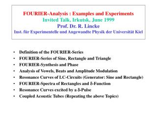
FOURIER-Analysis : Examples and Experiments Invited Talk, Irkutsk, June 1999 Prof. Dr. R. Lincke Inst. für Experimentelle und Angewandte Physik der Universität Kiel. Definition of the FOURIER-Series FOURIER-Series of Sine, Rectangle and Triangle FOURIER-Synthesis and Phase

E N D
FOURIER-Analysis : Examples and ExperimentsInvited Talk, Irkutsk, June 1999Prof. Dr. R. LinckeInst. für Experimentelle und Angewandte Physik der Universität Kiel • Definition of the FOURIER-Series • FOURIER-Series of Sine, Rectangle and Triangle • FOURIER-Synthesis and Phase • Analysis of Vowels, Beats and Amplitude Modulation • Resonance Curves of LC-Circuits (Generator: Sine and Rectangle) • FOURIER-Spectra of Rectangles and -Function • Resonance Curves excited by a -Pulse • Coupled Acoustic Tubes (Repeating the above Topics)
FOURIER-Analysis of Some Typical Signals A) 3 complete periods of a harmonic oscillation in the window result in a single contribution at the 3rd harmonic. B) A rectangular signal with the on/off ratio 1:1 contains only the odd harmonics i = 1, 3, 5 .. with Ai=1/i. C) A triangular signal also contains only odd harmonics, but now with Ai=1/i2. A) B) C)
FOURIER-Synthesis The FOURIER coefficients determined in the foregoing are now recombined to recover the signal: A) Ak = 0.9/k with k = 1, 3, 5, ··· yields a rectangle. B) Bk = 0.9/k with k = 1,-3, 5, -7 again produces a rectangle, but now with different phase. C) Bk = 0.573/k2 yields a triangle. A) B) C)
FOURIER-Analysis of Vowels These are real microphone recordings. Left: the vowel A with many harmonics. Right: the vowel U, which is nearly harmonic and contains only two important partial waves. The period of the acoustic signal was always chosen as window for the analysis.
FOURIER-Analysis of Beats Definition of beats : Ys = y1 ·cos(1·t) + y2 ·cos(2·t) Beats are strictly periodic only if the frequencies 1 and 2 are commensurable, i.e. if 1 = n ·(2- 1 ) with n = 1,2,3,4,···. In the left recording, this condition is fulfilled, and the Fourier spectrum contains only the contributions 1 and 2 (with frequency and amplitude). For the right - not strictly periodic - signal there existists no FOURIER series.
Amplitude Modulation (Sine) Definition:YAM = [yt + ym·sin(m·t)]·sin(t·t)(t=carrier, m=modulation) Rearranging :YAM = yt·sin(t·t)] + ½·ym ·cos[(t - m)·t] - ½·ym ·cos[(t + m)·t] The spectrum of an amplitude modu- lation thus contains the unmodified carrier tas well asa lower an upper side band with frequencies t - m andt + m. In order for the whole signal to be strictly periodic, it was again made sure that tundm are commensu- rate (compare Beats).
Amplitude Modulation (Rectangle) Here we use a rectangular signal (50:50) for the amplitude modulation. This rectangle contains the odd FOURIER components An ~ 1/n² with n = 1, 3, 5 ··. They reappear as lower and upper side bands in the FOURIER spectrum of the amplitude modulation.
Measuring C from the Discharge Time An important application for the FOURIER analysis will be the electromagnetic LC-circuit. For this we measure the capacity using the time constant of discharge: Three time constants R·C correspond to a faktor e-3 = 0,0498, i.e. the voltage must decay from 2000 to a value of 99,6. Here we get 3 R·C = 966 ms. Using the input impedance of UNIMESS R = 1 M , we get C = 0,322F. This is in perfect agreement with an independent precision measurement!
Measuring L from the Decay Time Here we measure the inductance from the decay time of the current through the coil: The time constant T = L/R corresponds to a factor e-1 = 0,368, i.e. the voltage over the shunt must decay from 1900 to 699. We measure L/R = 2,82 ms. With the ohmic resistance of the coil equal to 11,26 and the shunt equal to 2,74 , there results L = 39,5 mH. This is 5% larger than obtained from a precision measurement. 8,2 2,74
Damped LC Oscillations After charging the capacitor to 12V, it is being discharged by the coil: The program triggers on the falling slope and records the damped oscillation. The 6 measured periods correspond to 4.12 ms or = 1456 Hz. With L = 37.75 mH and C = 0.323 F we expected = 1/2· L·C = 1441 Hz. From the two marked amplitudes one calculates the damping constant = ln(1748/776)/(4.77-0.65) ·1000 = 197. From theory one expects = R/2L. With R = 11.26 and L = 37.75 mH this yields = 149. The reason for this error of 32% is not clear.
LC Resonance Curve with Sinusoidal Driver The program sweeps the frequency of the generator FD4E and measures and plots the rectified and averaged voltage. With the FD4E set to a sinusoidal driving voltage, the spectrum contains only the resonance at = 1/2· L·C. With L = 37.75 mH and C = 0.323 F it should lie at 1441 Hz.
LC Resonance : Secondary Circuits If one couples a second LC circuit S (with nomi-nally equal L and C) inductively to the primary circuit P, then the resonance splits up. If one couples a 3rd circuit T onto S one obtains a 3rd maximum in the curve (PST). If, however, one adds the 3rd circuit symmetrically to the other side of the primäry circuit (SPS), it behaves like a 2nd secondary circuit, and the curve has two maxima (now the phases are equal!). 3 Kreise: PST 2 Kreise: PS
LC Resonance Curve with Rectangular Driver The program sweeps the frequency of the function generator FD4E and records the rectified signal across R. With the function generator set to rectan-gular output, each harmonic (Ak=1/k2) produces its resonance at k times the frequency (see below). The partial waves thus are physically real, not just mathema-tical tricks!
FOURIER-Analysis of Rectangles • Sequence of rectangular signals with decreasing on/off ratios : • rectangle 50% Ai = 1/i, only odd harmonics • rectangle 10% the 10th harmonic is missing • rectangle 1% the 100th harmonic is missing • -function white continuum to
Resonance Curves with -Pulses The spectrum of a delta pulse is a white cont- tinuum. The voltage divider (R=10 kOhm and the impedance of the LC circuit) passes the partial waves according to ist frequency depen-dent characteristic, i.e. the LC resonance curve. The time function is a damped oscillation (or beats with coupled secondary circuit).
Acoustic Pipes: an Alternative to LC Circuits Coupled acoustic pipes, excited with a loudspeaker, show many of the features discussed in connection with LC circuits. LS : loudspeaker M : microphone with precision rectifier R1 and R2 : perspex pipes with distance x. The detailed form of the inten- sity curve depends strongly on the position of the microphone. Because of the end correction, the measured fundamental wave- length is slightly larger than 1 m corresponding to 0 = 341 Hz. One pipe of 50 cm
Acoustic Pipes: Coupling Splits the Resonance 5 mm 20 mm A systematic variation of the separation x between the pipes gives the frequencies for the upper and lower maximum shown in the right diagram. At large separations, the curves converge towards 633 Hz, for small x towards 333 Hz. (Compare the resonances of pipes of length L and 2L). f+ f- x
Acoustic Pipes: Phases in Maxima These are 2-channel recordings made at the upper and lower maximum of the resonance crve (x =3 mm) : 569 Hz 650 Hz In the lower branch the oscillations are in phase, in the upper in opposite phase
Acoustic Pipes: Frequency Separation Now we excite the pipes by discharging a capacitor through the loudspeaker (-Funktion). f+ fs f - The time signal shows damped beats. If one measures the beat frequency fs one obtains the difference between the upper and the lower frequency f+- f -in the resonance curve. A FOURIER analysis of the time function recovers the resonance curve.