Download
1 / 1
10 likes | 126 Views
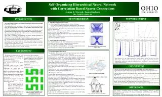
This research work presents a novel algorithm for a Self-Organizing Hierarchical Neural Network that incorporates correlation-based sparse connections. The network design and output generation process are detailed, showcasing the correlation and connection determination methods. Training the network using a Hybrid algorithm with considerations for sparse connectivity is covered. The hierarchical structure aims for invariant representations across a sequence of images, with a focus on self-organization through correlation and sparsity. This approach has potential applications in various fields such as surveillance, traffic monitoring, and rescue missions. The sparsity of connections reduces computational complexity and enables hardware implementation. The structured self-organization facilitates feature selection and memory association, building sequential memories of spatio-temporal patterns. The network's hierarchical layers progressively develop abstract feature representations, culminating in object, scene, concept, and skill representations.

E N D
Fig.6 Growth of Neighborhood Connections Fig.7 Network Activity in the Layers Wiring area Fig.3 Correlation/PDF Example Fig.1 2-D Network Example of the standard SOM[2], Fritzke’s GNG, and the Hybrid network Self-Organizing Hierarchical Neural Network with Correlation Based Sparse Connections Janusz A. Starzyk, James Graham Ohio University, Athens, OH NETWORK DESIGN NETWORK OUTPUT INTRODUCTION • Algorithm Operation Overview • Once data is input, correlation is performed on the provided images. • This tells how each pixel is correlated to all other pixels in the input space. • Feedback correlation is also determined by offsetting the data 1 time step. • Next, the first layer’s input and feedback connectivity structures are determined from the correlation data. • Then training is performed using the Hybrid algorithm with some changes needed to account for the sparse connectivity. • Once training is complete, the entire set of images is presented to the network and the output is determined. • Output is used to determine correlation data needed to construct the next layer. • The process is repeated in all layers. • Performing the correlation: • The simple 1D nature of the pixel value input does not lend itself to useful correlation, therefore, we perform a multi-dimentional correlations. • Fig. 2 presents a 3D correlation vs. a 10D correlation. • For our work 10D was deemed sufficient, even though at higher dimensionality even the slight curves visible in the 10D images disappear. • Determining the connections: • Now that pixel correlations are known, the input connections can be determined. • The concept is similar to Fig. 4, but in a 3D sense. • For the first layer each pixel has a neuron “positioned” directly above. This is not necessarily the case in higher layers and a composite correlation of the surrounding neurons is used. To determine input connections, positive portions of the correlation are treated as a probability distribution function (PDF). • The PDF is translated into a CDF function and used to randomly select a number of points in the correlated region. • The actual number of points is determined randomly about a mean based upon the size of each layer - a predefined constant. • Fig. 3 shows an example of the correlation about pixel 132 in a simple 18x14 pixel image set. • Ideally, this will result in an overlapping connectivity structure that will end with the type of forward connectivity shown in Fig. 4. • Training the Network: • To train a layer, images are presented in sequential order. • Next, winning neurons are determined based on how close their weights are to their input values (as in the Hybrid and GNG networks). • Neighbors are chosen in a similar manner to the GNG network, in that their next nearest neighbor becomes a neighbor. However, to be a neighbor a node must share at least some percentage of the same input connections (usually 50%). • The winning neurons are then evaluated to see if they are strong enough to fire (taking feedback into account as well). • Feedback may be able to activate a neuron with insufficient input activation. • At the end of training the network is evaluated to determine the output for the known images. • The output data is then correlated and presented to the layer building subroutine to construct the next layer. • In this way the feed-forward and feedback connections are created leading toward invariant representations for a sequence of images. • This work attempts to build a self-organized hierarchical structure with correlation based sparse connectivity. • Self-organizing networks, hierarchical or otherwise, have been researched for many years, and have applications in such areas as: surveillance, traffic monitoring, flight control, rescue mission, etc. • The sparsity of connections greatly reduces computational overhead and facilitates eventual hardware implementation of a network based on the proposed algorithm. • Sparse connection are provided only to those neurons on a lower level of hierarchy that are most correlated to each other. • This yields a structured self-organization of feature selection, providing an effective tool to associate different regions of memory. • Correlation over the time and space produces wiring to build sequential memories that store spatio-temporal patterns of sensory representations and motor skills. • The neural network representations are built using spatio-temporal associations observed locally in the input space and extended upwards through the hierarchy towards associations in the feature space. • “Higher” layers form increasingly abstract feature representations, eventually representing entire objects, scenes, concepts, and skills. Fig.5 Five Layers of Network Activity Fig.2 Multi-Dimentional Correlation (3D vs. 10D) BACKGROUND • The design for our network was based on Fritzke’s GNG [1]. It was modified to not rely on parameters for adjusting the error or weights of nodes. • We refer to it as a hybrid network. • Some relevant features of the Hybrid Network are: • The hybrid method starts with a random pre-generated network of a fixed size. • Connections get “stiffer” with age, making their weights harder to change. • Error is calculated after the node position updates rather than before as in Fritzke’s. • Weight adjustment and error distribution are based on “Force” calculations rather than constants. • Neighborhood connections are removed only under the following conditions (instead of all the time). • When a connection is added and there is another connection of length 2x greater than the node’s average connection length. • When a node is moved it looses its existing connections This work took the Hybrid algorithm and expanded upon it. Our self-organizing hierarchical network is designed to allow • for invariant object recognition. • In a typical NN all of the input pixels would be connected to all of the neurons. This is an inefficient use of resources. • Instead, we implemented: • Correlation based sparse input connections. • Hierarchical expanding layers for building invariance. Above, Figures 5, 6, and 7 depict the results of training a 5 layer network on a small set of 252 pixel images. Figure 5 shows the actual layer outputs. Figure 6 shows the growth in neighborhood connectivity within the individual layers. And figure 7 shows actual neuron activity within the layers. CONCLUSIONS • We have successfully implemented a method for determining sparse input connectivity. • And combined it with the hybrid self-organizing structure described in the background section. • The networks was then expanded and adjusted to work as a hierarchical network. • We have shown from the results in Figure 6 and 7 that this work lends itself to forming invariant representations. • The next step will be implementing feedback to form the invariances and ensuring that the algorithm is able to handle larger images than those already in use. • Some early testing of larger image sets consisting of higher resolution images has shown that there are some bottlenecks in the program due to the conflict between sparse matrices (needed to conserve memory for large matrices) and the slowdown they cause when being accessed. • Also, there is the possibility of implementing lateral input connections to improve the selection of winning neurons. REFERENCES [1] B. Fritzke, “A Growing Neural Gas Network Learns Topologies,” Advances in Neural Information Processing Systems 7, G. Tesauro, D.S. Toretzky, and T.K. Leen, (eds.), MIT Press, Cambridge MA, 1995. [2] T. Kohonen, "The Self-Organizing map", Proc. of IEEE, 78:1464-1480, 1990. Fig.4 Network Connectivity Example