Download
1 / 16
160 likes | 318 Views
State-of-the-art physical models for calculating atmospheric pressure loading effects. Dudy D. Wijaya , Böhm J., Schindelegger M., Karbon M., Schuh H. Institute of Geodesy and Geophysics, TU Vienna. Geodätische Woche 2010 5-7 October, 2010 - K ö ln, Germany.

E N D
State-of-the-art physical models for calculating atmospheric pressure loading effects Dudy D. Wijaya, Böhm J., Schindelegger M., Karbon M., Schuh H. Institute of Geodesy and Geophysics, TU Vienna Geodätische Woche 2010 5-7 October, 2010 - Köln, Germany
1. Introduction: The Project GGOS Atmosphere at TU Vienna • Purpose and significance Provide a detailed and comprehensive knowledge how the atmosphere affects observations of the three pillars of geodesy: geometry, gravity field & rotation Contribute to a better understanding of the system Earth • Main goals • Determine consistent and homogeneous models for • Atmospheric Propagation Delay (Delay) : Johannes Böhm (project leader) • Atmospheric Angular Momentum (AAM) : Michael Schindelegger • Atmospheric Gravity Field Coefficients (AGC) : Maria Karbon • Atmospheric Pressure Loading (APL) : Dudy D. Wijaya http://ggosatm.hg.tuwien.ac.at/
2 weeks Global atmospheric pressure circulation DOY in 1980 15 60 30 45 75 90 The Earth’s crust 1. Introduction: Atmospheric pressure loading (APL) • The mechanism of atmospheric loading • Characteristics of atmospheric loading Onsala - Sweden (Lat: 57o N) Pressure (mbar) Vertical displ. (mm) (van Dam & Wahr, 1987) Boulder - USA (Lat: 40o N) Pressure (mbar) Deformation of the Earth’s crust Pressure variations Vertical displ. (mm) 15 60 30 45 75 90 DOY in 1980
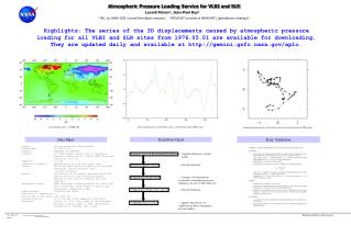
1. Introduction: Atmospheric pressure loading (APL) • Characteristics of atmospheric loading Radial displacement at August 1, 2008, 00 UT • Rule of thumb : • 10 hPa ≈ 3 mm radial displacement • Temporal variations : • annual, one to few weeks, diurnal, • semidiurnal mm • APL Service • Petrov & Boy : http://gemini.gsfc.nasa.gov/aplo/ • H. –G. Scherneck : http://www.oso.chalmers.se/~hgs/apload.html • van Dam & Gegout : http://www.sbl.statkart.no/aboutloading/ • TU Vienna : http://ggosatm.hg.tuwien.ac.at/LOADING/VERSION1/
Global pressure data Atmospheric tides Oceanic response Pressure variations 2. APL Modeling : The basic components of APL determination • The IERS recommendation: Geophysical model Reference pressure The Green’s function (weight function) Surface pressure • The basic components Earth model geometry, mechanical properties, rheology Load Love Numbers The Green’s function & Theory & mathematical model elastic theory, boundary conditions, extension of load Tidal & non-Tidal Surface displacements U
2. APL Modeling : Load Love Numbers and the Green‘s functions (a) • Determination of Load Love Numbers (hn, ln, kn) The SNREI Earth model : Preliminary Earth Reference Model (PREM), Gutenberg-Bullen Model (GB-model) Fundamental theory : Free oscillations of the Earth & elastic-gravitation theory Harmonic degree n : 10000 • Definition of the radial Green’s function (GR) PREM model GB model Love number Legendre (angular distance in degree) Formalism of the horizontal Green’s function (Gh) is similar
2. APL Modeling : Load Love Numbers and the Green‘s functions (b) • Effect of different Earth models on APL displacements The difference of APL displacements for some VLBI sites (PREM minus GB model) Radial displacements Eastward displacements WETTZELL ALGOPARK MON-PEAK • The difference of the displacements due to the choice of a specific Earth model is small (< 1mm). • We choose PREM model for our operational solutions.
2. APL Modeling : Definition of reference pressure • Global Reference Pressure (GRP) Reference pressure GRP error (hPa) • GRP model: • is based on the ECMWF 40 re-analysis (ERA-40) data • (monthly means) • provides a reference pressure value at any point • is suitable for various applications GRP memo, GRP data and MATLAB/Fortran codes can be found at http://ggosatm.hg.tuwien.ac.at/LOADING/REFPRES/ Schuh et al. (2010)
2. APL Modeling : Surface pressure & non-tidal displacements (a) • European Centre for Medium-range Weather Forecasts (ECMWF) Lat=0, Lon=50 Surface pressure • Temporal resolution : 00, 06, 12, 18 UTC • Spatial resolution : 1o x 1o • Problem of atmospheric pressure tides in the 6h fields • Representation of atmospheric tide signals is • not accurate. • The 6h fields do not permit proper resolution of the • S2 tide. • Atmospheric pressure signals S1/S2 should be • removed and non-tidal APL displacements • should be calculated (Ray & Ponte, 2003). S2 S1 Spectra x 1012 (Pa2/Hz)
2. APL Modeling : Surface pressure & non-tidal displacements (a) • European Centre for Medium-range Weather Forecasts (ECMWF) Lat=0, Lon=50 Surface pressure • Temporal resolution : 00, 06, 12, 18 UTC • Spatial resolution : 1o x 1o With (wrong) tide Tide free • Problem of atmospheric pressure tides in the 6h fields • Representation of atmospheric tide signals is • not accurate. • The 6h fields do not permit proper resolution of the • S2 tide. • Atmospheric pressure signals S1/S2 should be • removed and non-tidal APL displacements • should be calculated (Ray & Ponte, 2003). S2 S1 Spectra x 1012 (Pa2/Hz) Reduced S1/S2 signals
2. APL Modeling : Surface pressure & non-tidal displacements (b) • Amplitude spectra of non-tidal displacements at WETTZELL Radial displacements With (wrong) tide Tide free S1 S2 Spectra x 105 (mm2/Hz) Eastward displacements S1 S2 Spectra x 105 (mm2/Hz)
2. APL Modeling : Surface pressure & non-tidal displacements (c) • Non-tidal displacements at WETTZELL and ALGOPARK WETT: Eastward displ. WETT: Radial displ. Petrov & Boy Vienna ALGO: Eastward displ. ALGO: Radial displ. Differences between Petrov & Boy and Vienna models are less than 10 % of total displacements
2. APL Modeling : Tidal displacements (a) • Three-hourly surface pressure from ECMWF (2005-2009) Lat=0, Lon=50 • Better representation of atmospheric tide signals • The 3h fields permit proper resolution of S2 and • ter-diurnal S3 tides S1 S2 S3 S4 Amplitude spectra (Pa2/Hz) • Trigonometric model for tidal displacements • Pressure tide model: Convolution with Green’s functions • Tidal displacements model:
2. APL Modeling : Tidal displacements (b) • Tidal displacements at WETTZELL and ALGOPARK WETT: Eastward displ. WETT: Radial displ. Petrov&Boy Vienna Van Dam ALGO: Eastward displ. ALGO: Radial displ. Differences between three models are less than 50 % of total displacements
3. Status of APL service at TU Vienna • Current status • Tidal and non-tidal displacements provided for all VLBI sites from 1980 till now. • Daily calculation (at 08:15 GMT+2). • Reference frame: Center of Mass (CM). • Next plans • Recalculation of Love numbers and the Green’s functions. • Improvement of S1/S2 tide corrections and oceanic response. • Tidal and non-tidal displacements provided for the nodes of a global 1 degree grid. • Reference frame: Center of Mass (CM) & Center of the solid Earth (CE). Download APL correction at http://ggosatm.hg.tuwien.ac.at/LOADING/VERSION1/
4. Summary, conclusion and future investigations • Summary and conclusion • State-of-the-art physical models for APL calculations have been presented and validated with results • from other providers. • Differences between Petrov & Boy and Vienna results are very small, less than 10 % of the APL • displacements (~20 mm) • Treatment of oceanic response was not discussed in this presentation. In the calculation we assume • that the oceanic response follows the inverted barometer principle. • REMARKS: if the APL displacements remain uncorrected in the analysis of space geodetic data it can • systematically affect other parameters as was shown by Dach et al. (2009) for GPS and Boehm et al. • (2010) for VLBVI. • Future investigations • Further improvements regarding theoretical and technical aspects will be done. • Thorough validations by VLBI observations and other space geodetic observations will be carried out.