Expected values, covariance, correlation and expected values
Expected values, covariance, correlation and expected values. Introduction to Bivariate Regression . Does talking about politics cause people to be more interested in politics? Or does an interest in politics cause people to talk about politics?. Is this a causal relationship?.

Expected values, covariance, correlation and expected values
E N D
Presentation Transcript
Expected values, covariance, correlation and expected values Introduction to Bivariate Regression
Does talking about politics cause people to be more interested in politics? Or does an interest in politics cause people to talk about politics?
Is this a causal relationship? Talking about politics Interest in Politics Talking about politics Interest in Politics
How often do you talk about politics? Times/Week Freq. Percent Cum. 0 162 11.58 11.58 1 231 16.51 28.09 2 233 16.65 44.75 3 226 16.15 60.9 4 175 12.51 73.41 5 148 10.58 83.99 6 47 3.36 87.35 7 177 12.65 100 Total 1399 100 Data=ANES, Stata code: tab talkpol
How interested are you in politics? Frequency Percent Cumulative 1. Not interested at all 87 6.3 6.3 2. Slightly interested 199 14.42 20.72 3. Moderately interested 521 37.75 58.48 4. Very interested 409 29.64 88.12 5. Extremely interested 164 11.88 100 Total 1380 100 data=ANES, Statacode: tab intpol
Review standard deviation and variance • Variance: for each unit or observation, it is the distance from the mean squared and then divide by the number of units. • Standard deviation – square root of variance • since variance is in squared units, it doesn't’t make any sense. The standard deviation can be understood in terms of the original measurement unit
Calculating variance and standard deviations Obs. Prestige Deviation^2 1 82 1177.18 2 83 1246.8 3 90 1790.14 4 76 801.46 5 90 1790.14 6 87 1545.28 7 93 2053 8 90 1790.14 9 52 18.58 10 88 1624.9 11 57 86.68 12 89 1706.52 13 97 2431.48 14 59 127.92 15 73 640.6 R code: Library(car) data(Duncan) attach(Duncan) plot(education, prestige, main="Deviation from the Mean", ylab="Prestige", xlab="Education Attainment") segments(education, mean(prestige), education, prestige) abline(h=mean(prestige))
Review: Units, mean, variance and standard deviation Variable Obs. Mean Variance Std. Dev. Talking politics 1399 3.1 4.7 2.18 Interest politics 1380 3.26 1.1 1.05
Expected value v. probability • If our population set of numbers is: 1,1,3,3,17, then the expected value is 5, even though P(5) = 0. • Suppose we know that E(X) = 5 with the equation y = 5 + 7x. • What is E(Y)?
Expected values Interest in politics Missing 26 Obs 1380 Mean 3.26 Std. Dev. 1.048 Var 1.099 What is the expected value? What is the range? Mode? Why are there 26 missing? Talk politics Missing 7 Obs 1399 Mean 3.099 Std. Dev. 2.177 Variance 4.737 What is the expected value? Why is the standard deviation and variance so high?
Causation • Time ordering • Covariation
Co-variation from variation? • (xi - xmean)^2/n average distance between the mean of x and each x value, squared • aka (xi - xmean) (xi - xmean)/n
Covariation? (xi - xmean) * (yi - ymean) / n-1
Covariation • covariance can take any value • negative infinity to positive infinity
Intuitive explanation (xi - xmean) * (yi - ymean) / n-1 • When x and y are high at the same time and x and y are low at the same time, then the covariance is positive • They are both higher than their means and so the products being added together are positive
Intuitive explanation (xi - xmean) * (yi - ymean) / n-1 • When x is low when y is high and vice versa, then the covariance is negative • They are both higher than their means and so the products being added together are negative
Plot showing negative covariance R code: library(foreign) #Choose the file `class_qog.dta' myFile <- file.choose() dat <- read.dta(myFile,header=TRUE) attach(dat) #Make Scatterplot scatterplot(wdi_mort~gle_gdp, reg.line=lm, smooth=TRUE, spread=TRUE, boxplots='xy', span=0.5, data=dat) Stata Code: twoway (lfitci wdi_mort gle_gdp) (scatter wdi_mort gle_gdp)
Intuitive explanation (xi - xmean) * (yi - ymean) / n • When sometimes: • x and y are high at the same time and x and y are low at the same time • And about half of the other time • x is low when y is high and vice versa • Then the covariance is about 0 • High positive numbers are added to high negative numbers
Covariance is a function of… • Variance (standard deviation) of x • Variance (standard deviation) of y • Relationship between x and y
How can you compare a covariance of 132 and 134,847? • 134, 847 could be high variance of x, high variance of y, high variance of both variables, or a high relationship between x and y? • Not that helpful?
How can you change the covariance to a number that tells you only the magnitude of the relationship between x and y? • Divide by the standard deviation of x * the standard deviation of y • Correlation = (x-xmean)*(y-ymean) /Sd(x) * sd (y) • Pearson r ranges from -1 to +1 • Weak correlation = .1 • moderate correlation = .4 • strong correlation = .7