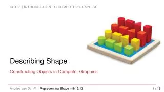
Describing Shape
Describing Shape. Constructing Objects in Computer Graphics. 2D Object Definition (1/3). Lines and polylines: Polylines: lines drawn between ordered points A closed polyline is a polygon, a simple polygon has no self-intersections Convex and concave polygons:

Describing Shape
E N D
Presentation Transcript
Describing Shape Constructing Objects in Computer Graphics Representing Shape – 9/12/13 / 16
2D Object Definition (1/3) • Lines and polylines: • Polylines: lines drawn between ordered points • A closed polyline is a polygon, a simple polygon has no self-intersections • Convex and concave polygons: • Convex: Line between any two points is inside polygon • Concave: At least one line between two points crosses outside polygon not closed, simple polyline simple polygon, closed polyline not simple polygon, closed polyline convex concave Representing Shape – 9/12/13 / 16
2D Object Definition (2/3) • Special Polygons: • Circles: • Set of all points equidistant from one point called the center • The distance from the center is the radius r • The equation for a circle centered at (0, 0) is r2= x2+ y2 Rectangle Square Triangle (x, y) (0, y) r (0, x) (0, 0) Representing Shape – 9/12/13 / 16
6 6 5 5 4 4 3 3 2 2 1 1 0 0 1 2 3 4 5 6 7 8 9 10 10 1 2 3 4 5 6 7 8 9 2D Object Definition (3/3) • A circle can be approximated by a polygon with many sides. • Axis aligned ellipse: a circle scaled in the x and/or y direction Scaled by a factor of 2 in the x direction and not scaled in the y direction. Width changes from 3.5 to 7. Representing Shape – 9/12/13 / 16
Representing Shape • Vertex and edge tables: • General purpose, minimal overhead, reasonably efficient • Each vertex listed once • Each edge is an ordered pair of indices to the vertex list • Sufficient to draw shape and perform simple operations (transforms, point inside/outside) • Edges listed in counterclockwise order by convention E3 E2 V4 V2 V3 E4 E1 E0 V0 V1 Representing Shape – 9/12/13 / 16
Splines (1/5) - Representing General Curves • We can represent any polyline with vertices and edges. What about curves? • Don’t want to store curves as raster graphics (aliasing, not scalable, memory intensive). We need a more efficient mathematical representation • Store control points in a list, find some way of smoothly interpolating between them • Closely related to curve-fitting of data, done by hand with “French curves”, or by computation • Piecewise Linear Approximation • Not smooth, looks awful without many control points • Trigonometric functions • Difficult to manipulate and control, computationally expensive to compute • Higher order polynomials • Relatively cheap to compute, only slightly more difficult to operate on than polylines Representing Shape – 9/12/13 / 16
Splines (2/5) – Spline Types and Uses • Polynomial interpolation is typically used. Splines are parametric curves governed by control points or control vectors, third or higher order • Used early on in automobile and aircraft industry to achieve smoothness – even small differences can make a big difference in efficiency and look. • Used for: • Representing smooth shapes in 2D as outlines or in 3D using "patches" parameterized with two variables: s and t (see slide 12) • Animation paths for "tweening" between keyframes • Approximating "expensive" functions (polynomials are cheaper than log, sin, cos, etc.) V0 interpolating spline V3 V2 approximating spline V5 polyline approximation V1 V4 Splines still exist outside of computers. They’re now called flexible curves. Representing Shape – 9/12/13 / 16
Splines (3/5) – Hermite Curves • Polylines are linear (1st order polynomial) interpolations between points • Given points P and Q, line between the two is given by the parametric equation: • and t are called weighting functions of P and Q • Splines are higher order polynomial interpolations between points • Like linear interpolation, but with higher order weighting functions allowing better approximations/smoother curves • One representation - Hermite curves (Interpolating spline): • Determined by two control points P and Q, an initial tangent vector v and a final tangent vector w. • Satisfies: w v Representing Shape – 9/12/13 / 16
Splines (4/5) – Hermite Weighting Explained Polynomial weighting functions in Hermite curve equation • Polynomial splines have more complex weighting functions than lines • Coefficients for P and Q are now 3rd degree polynomials • At t = 0 • Coefficients of P is 1, all others 0 • Derivative of coefficient of v is 1, derivative of all others is 0 • At t = 1 • Coefficient of Q is 1, all others 0 • Derivative of coefficient of w is 1, derivative of all others 0 • Can be chained together to make more complex curves 1 Q’s Coefficient P’s Coefficient w’s coefficient v’s coefficient (0, 0) 1 Representing Shape – 9/12/13 / 16
Splines (5/5) – Bezier Curves • Bezier representation is similar to Hermite • 4 points instead of 2 points and 2 vectors • Initial position P1, tangent vector is • Final position P4, tangent vector is • This representation allows a spline to be stored as a list of vertices with some global parameters that describe the smoothness and continuity • Bezier splines are widely used (Adobe, Microsoft) for font definition • See chapters 23 and 24 for more on splines www.cs.brown.edu/exploratories/freeSoftware/repository/edu/brown/cs/exploratories/applets/bezierSplines/bezier_splines_guide.html Image credit: http://miphol.com/muse/2008/04/25/Bezier-courbes-anim.gif Representing Shape – 9/12/13 / 16
Bezier Curve Example // Define the control points GLfloat points[4][3] = { { -4.0, -4.0, 0.0}, { -2.0, 4.0, 0.0}, {2.0, -4.0, 0.0}, {4.0, 4.0, 0.0}}; // Create an “evaluator” to define the polynomial that will be used to generate vertices glMap1f(GL_MAP1_VERTEX_3, // type of object to be evaluated 0.0, // starting parameter value 1.0, // ending parameter value 3, // “stride”: how many values between one vector and the next 4, // number of control points &points[0][0]); // location of control point data glEnable(GL_MAP1_VERTEX_3); glBegin(GL_LINE_STRIP); // evaluate 30 points on the curve, displayed using a contiguous sequence of lines for (inti = 0; i <= 30; i++) glEvalCoord1f((GLfloat) i/30.0); // evenly spaced values between 0 and 1 glEnd(); Representing Shape – 9/12/13 / 16
“Vertices in Motion” - Object Definition • A line is drawn by tracing a point as it moves (1st dimension added) • A rectangle is drawn by tracing the vertices of a line as it moves perpendicularly to itself (2nd dimension added) • A rectangular prism is drawn by tracing the vertices of a rectangle as it moves perpendicularly to itself (3rd dimension) • A circle is drawn by tracing a point swinging at a fixed distance around a center point. Representing Shape – 9/12/13 / 16
Building 3D Primitives • Made out of 2D and 1D primitives • Triangles are commonly used • Many triangles used for a single object is a triangular mesh • Splines used to describe boundaries of "patches" – these can be "sewn together" to represent curved surfaces Image credit (Stanford Bunny): http://mech.fsv.cvut.cz/~dr/papers/Habil/img1007.gif Representing Shape – 9/12/13 / 16
Triangle Meshes • Most common representation of shape in three dimensions • All vertices of triangle are guaranteed to lie in one plane (not true for quadrilaterals or other polygons) • Uniformity makes it easy to perform mesh operations such as subdivision, simplification, transformation etc. • Many different ways to represent triangular meshes • See chapters 8 and 25 in book, en.wikipedia.org/wiki/polygon_mesh • Mesh transformation and deformation • Procedural generation techniques(upcoming labs on simulating terrain) Image credit: http://upload.wikimedia.org/wikipedia/commons/f/fb/Dolphin_triangle_mesh.png Representing Shape – 9/12/13 / 16
Triangular Mesh Representation • Vertex and face tables, analogous to 2D vertex and edge tables • Each vertex listed once, triangles listed as ordered triplets of indices into the vertex table • Edges inferred from triangles • It’s often useful to store associated faces with vertices (i.e. computing normals: vertex normal average of surrounding face normals) • Vertices listed in counter clockwise order in face table. • No longer just because of convention. CCW order differentiates front and back of face v4 v7 f11 v8 f10 f8 f9 v6 f0 v5 f2 f1 f3 v0 v1 v2 Diagram licensed under Creative Commons Attribution license. Created by Ben Herila based on http://upload.wikimedia.org/wikipedia/en/thumb/2/2d/Mesh_fv.jpg/500px-Mesh_fv.jpg Representing Shape – 9/12/13 / 16
Book Sections • Chapter 8 • Chapters 22 and 23 for splines (warning: pretty heavy math) • Chapter 24 for implicit shapes • Chapter 25 for meshes Representing Shape – 9/12/13 / 16