Download
1 / 53
530 likes | 719 Views
Next time. Student presentations Rationale Format. Presentations. Please limit to 5 min If you have a ppt, bring it in on a USB flash drive (preload please) Overview of your project (Why, Where) Approach or method (How) Results, output to discuss (if any at this time)

E N D
Next time • Student presentations • Rationale • Format
Presentations • Please limit to 5 min • If you have a ppt, bring it in on a USB flash drive (preload please) • Overview of your project (Why, Where) • Approach or method (How) • Results, output to discuss (if any at this time) • You will have time to answer one or two questions max
Audience • Please ask at least one question – I will keep track of this • You will also be evaluating each presenter based on a set of criteria • The evaluations will be returned to each speaker
Presentation evaluations • Rate the clarity and organization of the presentation. • How well did the project incorporate available GIS/spatial analysis techniques? • Suggestion to improve presentation or project: ______________________
Menu • 4:15 pm • 7 pies • 3 pep, 1 plain, 2 veg mix, 1 ass-meat • Diet Coke, Coke, Sprite • You may bring a dessert to share if you wish
CART and GIS RESM 575 Spring 2009 Lecture 15
CART “Tree modeling” • A local nonparametric model • Decision tree • Data driven This type of tree -> <- Not this one
CART approach • Identify thresholds in predictor variables that partition response data optimally • Result in decision rules associated with “suitability or probability of presence”
CART • Useful when the response variable is made up of several distinct, unordered classes • Not significantly affected by outliers (Verblya, 1987) • Regression trees • Used to predict numeric values • Classification trees • Used to predict classifications
Classification trees vs Regression trees • Classification trees • Should be used to predict habitat types • “Categorical data” • Regression trees • Could be used to predict abundances • “Numeric data”
CART (some general notes) • Tree models are overfitted first then reduced later • Various methods to reduce trees • 10fold optimization • GINI method
Methods for determining tree size • One standard error rule (with or without cross-validation). • Akaike's Information Criterion (classification trees only). • Mallow's Cp (regression trees only). • The Gini index • is a measure of impurity with values ranging from 0 to 1, where 0 represents total purity (all observations in the node are in one class) and 1 equals total impurity (all classes are equally represented in the node). • The reduction in the Gini index is measured as the impurity of a group before the split, minus the sum of the impurities of the two groups resulting from the split.
Evaluation Splus • The tree may be pruned using deviance or misclassification rate to evaluate the subtrees, or the tree my be shrunken.
Model Assessment – Kappa Analysis • Kappa can be used as a measure of agreement between model predictions and reality (Congalton 1991) or • to determine if the values contained in an error matrix represent a result significantly better than random (Jensen 1996). • Kappa is considered to be a reliable measure of accuracy if the z-score is significant (Fleiss 1973).
CART Advantages • Easy to interpret • Useful for non-linear, non-additive and hierarchical relationships • Possible to investigate variable importance • Pruning measures available for variable reduction • Accepts categorical data
CART Disadvantages • Somewhat computer intensive • Less powerful than parametric methods when response functions are simple • Requires multiple software
CART Software • CART by Salford Systems • Random forests • Its strengths are spotting outliers and anomalies in data, displaying proximity clusters, predicting future outcomes, identifying important predictors, discovering data patterns, replacing missing values with imputations, and providing insightful graphics. Additionally, it can provide clustering and density estimations. • SPLUS, R, JMP, SAS, etc
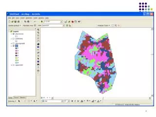
StatMod http://www.gis.usu.edu/~chrisg/avext/ • Goal: developed to help statistical modeling for ecologists • Helps perform logistic regression with SAS and GIS Or • Performs CART analysis with GIS • Provides graphical user interface and more…
Basics of StatMod Spatial Data in GIS Sample GIS Themes Set up Analysis Options Run Statistical Analysis Helps Read Output Back into GIS
Additional functions of StatMod • Helps user convert and resample data • Select random points • Perform Kappa analysis
StatMod installation • Simply copy statmod.avx into the c:/esri/av_gis30/arcview/ext32 directory
References Andersen, M. C., J. M. Watts, J. E. Freilich, S. R. Yool, G. I. Wakefield, J. F. McCauley, and P. B. Fahnestock. 2000. Regression-tree modeling of desert tortoise habitat in the central Mojave desert. Ecological Applications 10: 890-900. Breiman, L., J. H. Friedman, R. A. Olshen, and C. J. Stone. 1984. Classification and Regression Trees. Chapman & Hall, New York, New York, U.S.A. Carroll, C., W. J. Zielinski, and R. F. Noss. 1999. Using presence-absence data to build and test spatial habitat models for the fisher in the Klamath region, U.S.A. Conservation Biology 13: 1344-1359. Congalton, R. G. 1991. A review of assessing the accuracy of classifications of remotely sensed data. Remote Sensing of Environment 37:35-46. Fleiss, J. L. 1973. Statistical Methods for Rates and Proportions. John Wiley & Sons, Inc., New York, New York, USA. Hosmer, D. W., and S. Lemeshow. 1989. Applied Logistic Regression. John Wiley & Sons, Inc., New York, New York, USA. Jensen, J. R. 1996. Introductory Digital Image Processing: A Remote Sensing Perspective (Second edition). Prentice Hall, Inc., Upper Saddle River,New Jersey, USA. Miller, J.M. 2005. Incorporating Spatial Dependence in Predictive Vegetation Models: Residual Interpolation Methods. The Professional Geographer, 57(2): 169-184. Rejwan, C., N. C. Collins, L. J. Brunner, B. J. Shuter, and M. S. Ridgway. 1999. Tree regression analysis on the nesting habitat of smallmouth bass. Ecology 80: 341-348. RS/GIS Laboratories, Utah State University. 2003. Sagebrush Ecosystem Mapping using Landsat ETM, Final Report. Unpublished manuscript. Schadt, S. E. Revilla, T. Wiegand, F. Knauer, P. Kaczensky, U. Breitenmoser, L. Bufka, J. •ervený, P. Koubek, T. Huber, C. Staniša, and L. Trepl.2002. Assessing the suitability of central European landscapes for the reintroduction of Eurasian lynx. Journal of Applied Ecology 39: 189-203. Verbyla, D. L. 1987. Classification trees: a new discrimination tool. Canadian Journal of Forest Research 17: 1150-1152.