Download
1 / 38
380 likes | 467 Views
Learn about AXA Rosenberg's investment philosophy rooted in fundamental analysis and how rational investing maximizes returns while minimizing risk through linear algebra and optimization techniques.

E N D
Linear algebra and rational investing Mark Howard Director of Software Engineering Barr Rosenberg Research Center April 1, 2009
Background on the Firm • Founded in the US in 1985 to manage diversified equity portfolios • Global equity specialist within AXA Investment Managers’ multi-expert group of asset managers • Offices located in major financial centers around the world • Stable, committed team of 380 employees worldwide • 341 clients including pension funds, governments, endowments and foundations • $118 billion assets under management as of March 2008
AXA Rosenberg: Sample Client List * This client list is intended simply to indicate a sample of AXA Rosenberg's non-confidential clients; the selection of clients for the list is intended to demonstrate the range of our institutional client base both geographically and by type of institution (corporate, insurance, pension plans, universities, endowments, etc.). It is not known whether the listed clients approve or disapprove of the manager or the advisory services provided.
A Rational, Proven Foundation Fundamental Analysis Through Expert Systems “A time-tried investment principle…to discover and acquire undervalued individual securities as the result of comprehensive and expert statistical investigations.” – Graham & Dodd, 1934
Strategy Overview • Investment philosophy rooted in persistent economic principles • Fundamentally driven: Earnings Matter • Systematic security analysis and portfolio construction • Robust in different market environments • Globally consistent with low regional correlations Implementation Objective Subjective Company Fundamentals AlphaSource Technical Strategies or Factor Models
100% 75% 77.8% 59.1% 55.3% 50% 42.2% 41.6% 29.3% 25% 26.8% 18.4% 12.8% 11.5% 8.6% 6.7% 0% AXA Rosenberg Market -25% How Our Strategy Works: A Snapshot More future earnings… Valuation Model Identify most attractively priced stocks in each industry + Earnings Forecast Model Identify companies with superior year-ahead earnings in each industry = …result in superior performance Forecast Company Return 4 3 Risk Model 2 Maximize return with minimum deviation from the benchmark 1 0
Valuation Model Identify most attractively priced stocks • Classic arbitrage analysis — identify stocks selling for less than the sum of a company’s parts • Analogous to real estate appraisal • Four-step comparison of prices to company fundamentals: • Identify and value 170 distinct business lines • Capture market value for each financial statement item • Identify value of unique features • Compare sum of company’s parts to current stock price
Portfolios For our purposes a portfolio is an allocation of our assets to securities. For example if our universe of securities is s1,…snthen a portfolio is a vector x1,…,xnof numbers in [0,1] which sum up to 1. xi is the proportion of our assets invested in si
Returns If you bought stock s for a dollars and sold it for b dollars then the return on s is (b-a)/a … in other words the amount gained (or lost) per dollar spent. If you have a portfolio x1,…,xnof stocks s1,…,snwith returns r1,…,rnthen the portfolio return is
Expected returns Assume that we have some way to predict returns … our prediction for stock is . Then the predicted or expected portfolio return is . We will refer to this as E.
Risk Assume that for each pair of securities si,sjwe have a number between 0 and 1 which measures the covariance between the predicted returns of si and sj. The variance or risk of the portfolio is
Matrices If we let the (column) vector denote our portfolio, denote the (column) vector of expected returns, the covariance matrix, the expected portfolio return, and the variance of the portfolio then
Rational investing The goal of rational investing is to maximize the expected return while minimizing the risk. A fundamental result of modern portfolio theory (for which Harry Markowitz won the nobel prize in economics) is that this tradeoff is meaningful.
Optimizing portfolios For a given return the problem of minimizing the risk is a quadratic optimization problem. One efficient method of solving this is to use convex piecewise linear programming.
George Dantzig In 1939 George Dantzig was a graduate student in statistics at Berkeley. One day he was late for class and wrote down the two problems on the board.
George Dantzig A few days later when he took them to his professor’s office he apologized for being late as they were somewhat harder than the other problems, and asked if he still wanted them. The professor (the great statistician Jerzy Neyman) told him to just toss them on the desk.
George Dantzig Several weeks later Neyman excitedly came to Dantzig’s house to tell him that those weren’t homework problems, but two of the most notorious open problems in statistics.
Linear Programming A few years later Dantzig invented the simplex method for solving (piecewise) linear programming problems. A linear programming problem is one of the form minimize subject to
Linear Programming Here the linear equation is underspecified … in other words A usually has many more columns than rows, so many the equation has many solutions. The core of the simplex method is effectively Gaussian elimination.
Financial models Returns are very hard to predict. It is actually much easier to predict other variables, such as future earnings, which affect returns. Under the assumption that the market will eventually reward earnings this should be sufficient to produce a portfolio with superior returns.
Earnings Forecast Model Objective: Estimate of Forward Earnings Forecast of next year’s earnings FundamentalIndicators What can we tell about future earnings based on historic fundamentals? Market Participant Indicators What is the market telling usabout future earnings? • Profitability Measures • Trends in earnings, ROA, ROE, etc. • Operating Ratios • Margins, debt coverage, etc. • Analyst Forecasts • Earnings Revisions • Broker Recommendations • Prior Price Behavior
Financial models One common technique for predicting variables, such as future earnings, is to determine some collection of current variables such as book value, sales, etc., and to try to find a linear combination of these which is a reasonable approximation to the predicted value we are looking for.
Financial models A technique for doing this was invented by Gauss in 1795 (when he was 18), and is now known as the method of least squares, or linear regressions.
Regression Say that we think that future earnings is really a linear combination of m other current variables. Assume that are the values for these variables for security i and that is the value of future earnings. Then there should be such that is close to for most i. other words there should be m coefficients such that for any values of our variables
Regression One way to achieve this is take observations in the past and the actual values we are trying to predict and to find which minimize the sum of squares of differences between the predicted values and the actual values.
Regression A little math shows that this sum of squares is minimized by Where X is the matrix of variables.
Financial models If we have found a reasonable set of explanatory variables then we can use this linear functional to predict future earnings…in other words we can try to maximize future earnings instead of the more elusive future returns, and then rely on the market to reward those earnings with returns.
Factor Models Usually when managing large portfolios the goal is not to minimize the volatility of the portfolio, but rather to minimize the difference between the portfolio return and the market return. One way to do this is to identify market factors and take into consideration every security’s exposure to those factors.
Factor Models A classic example of a market factor is which industry a company is in. We enumerate all of the industries and for each company give it a number between 0 and 1 indicating how much of the company is in that industry.
Factor Models Once we have our factors we can use the same techniques as before to minimize the difference between the average exposure to each factor and the market’s average … so if there are economic forces which cause a particular factor to behave differently then we will track the difference.
Factor Models Factors are constructed by hand by thinking about economic forces, but once you have created what you think are reasonable factors you can use eigenvalue decomposition of the factor covariance matrix to create a more precise set of factors.
Solving equations It is very common in portfolio optimization to be faced with the problem of solving sequences of systems of linear equations
Solving equations Where each Ai+1 differs from Aiin only one column. The traditional way to solve Ax=b is to invert A, and use A-1b, but there are many matrices for which solving the equation is much easier than inverting the matrix (e.g.triangular matrices).
Solving equations One very useful computational technique is to factor A into matrices which are easy to solve, for example represent A = LU where L and U are easy to solve… then Ax=b is the same as L(Ux) = b, so if Ly = b and Ux = y then Ax=b.
Solving equations One very useful computational technique is to factor A into matrices which are easy to solve, for example represent A = LU where L is lower triangular and U is upper triangular … then Ax=b is the same as L(Ux) = b, so if Ly = b and Ux = y then Ax=b.
Solving equations It turns out that one can slightly complicate this and get factorizations of Ai with the property that the i+1th factorization is easily computable from the ith factorization and the difference between Ai+1and Ai, so solving the sequence of equations is fast.