Logic Programming (cont’d): Lists
160 likes | 293 Views
Logic Programming (cont’d): Lists. Lists in Prolog are represented by a functor (similar to cons in Scheme): The empty list is represented by the constant - [ ]. The term .(X , Xs ) represents a list of which X is the 1 st element and Xs is the rest of its elements.

Logic Programming (cont’d): Lists
E N D
Presentation Transcript
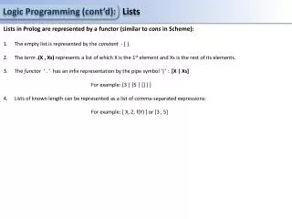
Logic Programming (cont’d): Lists Lists in Prolog are represented by a functor (similar to cons in Scheme): The empty list is represented by the constant - [ ]. The term .(X , Xs) represents a list of which X is the 1st element and Xs is the rest of its elements. The functor‘ . ’ has an infix representation by the pipe symbol ‘|’ : [X | Xs]For example: [3 | [5 | [] ] ] Lists of known length can be represented as a list of comma-separated expressions: For example: [ X, 2, f(Y) ] or [3 , 5]
Logic Programming (cont’d): Lists Example 1: Implementing a Context Free Grammar in PROLOG: Representation in PROLOG: s(Z) :- np(X),vp(Y),append(X,Y,Z). np(Z):- det(X),n(Y),append(X,Y,Z). vp(Z):- v(X),np(Y),append(X,Y,Z).vp(Z):- v(Z). det([the]).det([a]). n([woman]).n([man]). v([saw]). Q: What language does this CFG represent? ?- s([a,woman,saw,a,man]).true ?-s(X).X = [the,woman,saw,the,woman];X = [the,woman,saw,the,man];X = [the,woman,saw,a,woman];X = [the,woman,saw,a,man];X = [the,woman,saw]… ?-s([the,man|X]).X = [saw,the,woman];X = [saw,the,man];X = [saw,a,woman]… S NP VP Det N V NP VP Det N V NP | V a | the woman |man saw
Logic Programming (cont’d): Lists Example 1: Implementing a Context Free Grammar in PROLOG: Representation in PROLOG: S NP Adj VP Det N V NP VP Det N | DetAdj N vicious | marvelous V NP | V a | the woman |man saw s(Z) :- np(X),vp(Y),append(X,Y,Z). np(Z):- det(X),n(Y),append(X,Y,Z). vp(Z):- v(X),np(Y),append(X,Y,Z).vp(Z):- v(Z). det([the]).det([a]). n([woman]).n([man]). v([shoots]). s(Z) :- np(X),vp(Y),append(X,Y,Z). np(Z):- det(X),n(Y),append(X,Y,Z). np(Z):- det(X),adj(W),n(Y),append([X,W,Y],Z). adj([vicious]). adj([marvelous]). vp(Z):- v(X),np(Y),append(X,Y,Z).vp(Z):- v(Z). det([the]).det([a]). n([woman]).n([man]). v([shoots]). Q: How would we implement the modifications above?
Logic Programming (cont’d): Lists • Example 2: Determining the order of specific times • In logic programming, symbols have no values: ‘2’ and ‘9’ are names and not numbers. • We cannot use the < relation to compare the order of numbers (it is infinite!). • However, a finite ordered relation may be represented by positions in lists. • We would like to implement an ordered relation between pairs of the form (hour, weekday). % Type: Hour. % Signature: h(Hour)/1 % Example: h(18). % Type: Weekday. % Signature: d(Weekday)/1 % Example: d(Tue).
Logic Programming (cont’d): Lists • Example 2: Determining the order of specific times • In logic programming, symbols have no values: ‘2’ and ‘9’ are names and not numbers. • We cannot use the < relation to compare the order of numbers (it is infinite!). • However, a finite ordered relation may be represented by positions in lists. • We would like to implement an ordered relation between pairs of the form (hour, weekday). % Signature: weekday_list(List)/1 % Purpose: Holds the ordered list of week days. weekday_list([d('Sun'),d('Mon'),d('Tue'),d('Wed'),d('Thu'),d('Fri'),d('Sat')]). % Signature: hour_list(List)/1 % Purpose: Holds the ordered list of days hours. hour_list([h(0),h(1),h(2),h(3),h(4),h(5),h(6),h(7),h(8),h(9),h(10),h(11),h(12), h(13),h(14),h(15),h(16),h(17),h(18),h(19),h(20),h(21),h(22),h(23)]).
Logic Programming (cont’d): Lists Example 2: Determining the order of specific times hour_list([h(0),h(1),h(2),h(3),h(4),h(5),h(6),h(7),h(8),h(9),h(10),h(11),h(12), h(13),h(14),h(15),h(16),h(17),h(18),h(19),h(20),h(21),h(22),h(23)]). weekday_list([d('Sun'),d('Mon'),d('Tue'),d('Wed'),d('Thu'),d('Fri'),d('Sat')]). A predicate to identify hours: % Signature: is_hour?(Hour)/1 % Purpose: Succeeds iff Hour is an hour of the weekday. is_hour(h(H)) :- hour_list(Hour_list), member(h(H),Hour_list). An order relation between hours: % Signature: hour_order(H1,H2)/2 % Purpose: hour H1 precedes the hour H2 in some weekday. hour_order(h(H1),h(H2)) :- is_hour(h(H1)), is_hour(h(H2)), hour_list(Hour_list), precedes(h(H1),h(H2),Hour_list).
Logic Programming (cont’d): Lists Example 2: Determining the order of specific times hour_list([h(0),h(1),h(2),h(3),h(4),h(5),h(6),h(7),h(8),h(9),h(10),h(11),h(12), h(13),h(14),h(15),h(16),h(17),h(18),h(19),h(20),h(21),h(22),h(23)]). weekday_list([d('Sun'),d('Mon'),d('Tue'),d('Wed'),d('Thu'),d('Fri'),d('Sat')]). A predicate to identify weekdays: % Signature: is_weekday?(Day)/1 % Purpose: Success iff Weekday is a weekday of the week. is_weekday?(d(D)) :- weekday_list(Weekday_list), member(d(D),Weekday_list). An order relation between weekdays: % Signature: weekday_order(Weekday1,Weekday2)/2 % Purpose: Weekday1 precedes weekday2 % in some week. weekday_LT(d(D1),d(D2)) :- is_weekday(d(D1)), is_weekday(d(D2)), weekday_list(Weekday_list), precedes(d(D1),d(D2),Weekday_list).
Logic Programming (cont’d): Lists Example 2: Determining the order of specific times % Type: Time. % Signature: time(Hour,WeekDay)/2 % Example: time(h(18),d(Tue)). A predicate to identify times: % Signature: is_time?(Time)/1 % Purpose: Succeeds iff Time is an hour of some weekday. % Example: ? – is_time? (time(h(1),d(‘Sun’))). true. is_time?(time(h(H),d(D))) :- is_hour?(h(H)), is_weekday?(d(D)). An order relation between times: % Signature: time_LT(T1,T2)/2 % Purpose: The time T1 precedes the time T2 in the week. % Example: ?- time_order(time(h(5),d(‘Mon’)),time(h(1),d(‘Tue’)). % true. time_order(time(h(H1),d(D1)),time(h(H2),d(D2))) :- is_time(time(h(H1),d(D1))),is_time(time(h(H2),d(D2))),weekday_order(d(D1),d(D2)). time_order(time(h(H1),d(D)),time(h(H2),d(D))) :- is_time(time(h(H1),d(D))),is_time(time(h(H2),d(D))),hour_order(h(H1),h(H2)).
Logic Programming (cont’d): Lists Example 4: Merging sorted lists % Signature: lt(Obj1,Obj2)/2 % Purpose: Obj1 precedes Obj2 by some comparison criteria. lt(Time1,Time2) :- time_LT(Time1,Time2). % Signature: merge(Xs,Ys,Zs)/3 % Purpose: Zs is the sorted merge of the sorted lists Xs and Ys. Assumes % there a predicate "lt" of order between elements of Xs and Ys. merge([X|Xs],[Y|Ys],[X|Zs]) :- lt(X,Y), merge(Xs,[Y|Ys],Zs). %1 merge([X|Xs],[X|Ys],[X,X|Zs]) :- merge(Xs,Ys,Zs). %2 merge([X|Xs],[Y|Ys],[Y|Zs]) :- lt(Y,X), merge([X|Xs],Ys,Zs). %3 merge(Xs,[],Xs). %4 merge([],Ys,Ys). %5 ?- merge([time(h(5),d('Sun')),time(h(5),d('Mon'))], X, [time(h(2),d('Sun')),time(h(5),d('Sun')),time(h(5),d('Mon'))]). X = [time(h(2),d( 'Sun'))]
Logic Programming (cont’d): Lists Example 5: Merging sorted lists merge([X|Xs],[Y|Ys],[X|Zs]) :- lt(X,Y), merge(Xs,[Y|Ys],Zs). merge([X|Xs],[X|Ys],[X,X|Zs]) :- merge(Xs,Ys,Zs). merge([X|Xs],[Y|Ys],[Y|Zs]) :- lt(Y,X), merge([X|Xs],Ys,Zs). merge(Xs,[],Xs). merge([],Ys,Ys). ?-merge( [ time(h(1),d('Sun')), time(h(3),d('Wed')), time(h(5), d('Sat'))], [ time(h(2), d('Sun')), time(h(3),d('Wed'))], Xs) merge([t1,t3,t5],[t2,t3],Xs) {X_1=t1,Xs_1=[t3,t5], Y_1=t2,Ys_1=[t3], Xs=[t1|Zs_1]} 1 lt(t1,t2), merge([t3,t5],[t2,t3],Zs_1) 2 – failure branch… 3 – failure branch… * merge([t3,t5],[t2,t3],Zs_1) {X_2=t3,Xs_2=[t5], Y_2=t2, Ys_2=[t3], Zs_1=[t2|Zs_2]} 3 lt(t2,t3), merge([t3,t5],[t3],Zs_2) 2 – failure branch… 1 – failure branch… * merge([t3,t5],[t3],Zs_2) 1 – failure branch… {X_3=t3,Xs_3=[t5],Y_3=t3,Ys_3=[],Zs_2=[t3,t3|Zs_3]} 2 1 – failure branch… merge([t5],[],Zs_3) {Xs_4=[t5],Ys_4=[], Zs_3=[t5]} 4 true
Logic Programming (cont’d): Backtracking optimization • Example 7: Optimize the procedure merge. • When none of the first two params is [], only one of the rules can be valid, • Since either lt(Y,X), or lt(X,Y) or X==Y holds, exclusively. • Once one of the above holds, we can skip further rule selections. merge([X|Xs],[Y|Ys],[X|Zs]) :- lt(X,Y), !, merge(Xs,[Y|Ys],Zs). merge([X|Xs],[X|Ys],[X,X|Zs]) :- merge(Xs,Ys,Zs). merge([X|Xs],[Y|Ys],[Y|Zs]) :- lt(Y,X), merge([X|Xs],Ys,Zs). merge([t1,t3,t5],[t2,t3],Xs) lt(t1,t2), !,merge([t3,t5],[t2,t3],Zs_1) 3 – failure branch… 2 – failure branch… !, merge([t3,t5],[t2,t3],Zs_1) merge([t3,t5],[t2,t3],Zs_1)
Logic Programming (cont’d): Backtracking optimization The cut operator (!): Used to avoid redundant computations. ?- , A,, …, . Rule k: A :- B1, …Bi, !, Bi+1, …, Bn. Rule k+1: A :- … . … ?- A,, …, . Rule k Following selections of A rules are cut. ?- B1,…, Bi, !, Bi+1, …Bn,Q1’,…Qm’ * Further substitutions for goals before ‘!’ are cut. ?- !, Bi+1’, …Bn’,Q1’’,…Qn’’ ?- Bi+1’, …Bn’,Q1’’,…Qn’’ …
Logic Programming (cont’d): Backtracking optimization • Example 8: red VS green cuts. • Green cut: Helps optimizing the program by avoiding redundant computations. • Red cut: Omits possible solutions. • Red cuts are undesired, unless specifically required (E.g., to provide only the first solution). • Q: How many possible solutions does the following query have? ?- merge([],[],X). X = [];X = [] The query matches both facts 4 and 5: merge(Xs,[],Xs). merge([],Ys,Ys). To avoid this, we add ‘!’ to fact 4, rewriting it as a rule: merge(Xs,[],Xs):-!. merge([],Ys,Ys). A red cut! The number of solutions has changed!
Logic Programming (cont’d): Meta circular interpreter • Recall the second version of the meta-circular interpreter (seen in class): • Based on goals reduction, with explicit control of selection order (using a stack of goals). • Operates in two phases: • Preprocessing: The given program, P, is translated into a new program P’, which has a single predicate, rule, and consists of facts only. • Queries are applied to the new program using the procedure solve.
Logic Programming (cont’d): Meta circular interpreter Example 10: Applying the meta circular interpreter. member(X,[X|Xs]). member(X,[Y|Ys]) :- member(X,Ys). % Signature: rule(Head,BodyList)/2 rule(member(X,[X|Xs]),[]). rule(member(X,[Y|Ys]),[member(X,Ys)]). Preprocessing % Signature: solve(Goal)/1 % Purpose: Goal is true if it is true when posed to the original program P. % Precondition: rule/2 is defined for the program. solve(Goal) :- solve(Goal,[]). % Signature: solve(Goal,Rest_of_goals)/2 solve([],[]). % (Nothing to prove, empty stack - done). solve([],[G | Goals]) :- solve(G,Goals). % (Nothing to prove, non-empty stack - pop). solve([A|B],Goals) :- append(B,Goals,Goals1), solve(A,Goals1). % (List to prove – push cdr). solve(A,Goals) :- rule(A,B), solve(B,Goals).
solve(member(X, [a, b, c])) {Goal_1 = member(X, [a, b, c])} 1 solve(member(X, [a, b, c]), []) {A_2 = member(X, [a, b, c], Goals_1 = []} 4 rule(member(X, [a, b, c], B_2), solve(B_2, []) {X_3 = X, Y_3 = a,Ys_3 = [b, c], B_2 = [member(X, [b, c])]} Rule 2 rule {X = a, X_3 = a,Xs_3 = [b, c], B_2 = []} 1 solve([],[]) solve([member(X, [b, c])], []) {A_4 = member(X, [b, c]), B_4 = [], Goals_4 = []} 3 1 true append([], [], Goals1_4), solve(member(X, [b, c]), Goals1_4) {X = a} {Goals1_4 = []} Rule of append solve(member(X, [b, c]), []) {A_5 = member(X, [b, c]), Goals_5 = []} 4 rule(member(X,[b, c]), B_5), solve(B_5, []) … {X = b, X_6 = b, Xs_6 = [c], B_5 = []} 1 solve([],[]) 1 true {X = b}