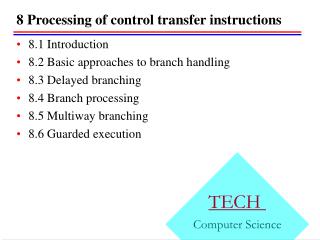
Understanding Control Transfer Instructions in Pipeline Architectures
Control transfer instructions are vital for maintaining the proper execution order within a CPU pipeline, especially in the presence of control dependencies that arise from branches. These dependencies can significantly affect execution efficiency. This chapter delves into the nature of control transfer instructions, including types of branches (conditional and unconditional), and their impact on dataflow. It highlights the role of the program counter (PC) in managing instruction flow and discusses performance measures, such as branch penalties and how they influence parallelism in code execution.


Understanding Control Transfer Instructions in Pipeline Architectures
E N D
Presentation Transcript
PROCESSING CONTROL TRANSFER INSTRUCTIONS Chapter No. 8 By Najma Ismat
Control Transfer Instructions • data hazards are a big enough problem that lots of resources have been devoted to over coming them but unfortunately, the real obstacle and limiting factor in maintaining a good rate of execution in a pipeline are control dependencies • branches are 1 out of every 5 or 6 inst. • In an n-issue processor, they’ll arrive n times faster • A “control dependence” determines the ordering of an instruction with respect to a branch instruction so that the non-branch instruction is executed only when it should be
Control Transfer Instructions • If an instruction is control dependent on a branch, it cannot be moved before the branch • They make sure instructions execute in order • Control dependencies preserve dataflow • Makes sure that instructions that produce results and consume them get the right data at the right time
How Control Instruction Can Be Defined? • Instructions normally fetched and executed from sequential memory locations • PC is the address of the current instruction, and nPC is the address of the next instruction (nPC = PC + 4) • Branches and control transfer instructions change nPC to something else • Branches modify, conditionally or unconditionally, the value of the PC.
Unconditional Branches i1 jmp 24 i3 i4 i5 i6 i7 i8 jmp 20 i10 10 14 jmp address 18 1c 20 24 28 2c 30 34
i1 jle 24 10 i1 jle 24 i3 i4 jmp 2c i6 i7 i8 i9 i10 14 18 1c i3 i4 jmp 2c i6 i7 20 24 28 2c i8 i9 i10 30 Basic blocks 34 Conditional jumps
Result State Concept • Architectures that supports result state approach are IBM/360 and 370, PDP-11, VAX, x86, Pentium, MC 68000, SPARC and PowerPC • the generation of the result state requires additional chip area • implementation for VLIW and superscalar architectures requires appropriate mechanisms to avoid multiple or out-of-order updating of the results state • multiple sets of flags or condition codes can be used
Example (Result State Concept) add r1, r2, r3 // r1<- r2 + r3 beq zero // test for result equals to zero and,if // ‘yes’ branch to location zero div r5, r4, r1 // r5 <- r4 / r1 . . . zero: // processing the case if divisor equals to // zero
Example (Result State Concept) teq r1 // test for (r1)=0 and update result state // accordingly beq zero // test for results equals to zero and, if yes, // branch to the location zero div r5, r4, r1 // r5 <- r4/ r1 . . . zero: // processing the case if divisor equals to // zero
The Direct Check Concept • Direct checking of a condition and a branch can be implemented in architectures in two ways: • use two separate instructions • First the result value is checked and compare and the result of the compare instruction is stored in the appropriate register • then the conditional branch instruction can be used to test outcome of the deposited test outcome and branch to the given location if the specified condition is met • use single instruction • a single instruction fulfils both testing and conditional branching
Example (Use Two Separate Instructions) add r1, r2, r3; // r1<- r2 + r3 cmpeq r7, r1; // r7 <- true, if (r1)=0, else NOP bt r7,zero // branch to ‘zero’:if (r7)=true, else NOP div r5, r4, r1 // r5 <- r4 / r1 . . . zero:
Example (Use Single Instruction) add r1, r2, r3 // r1<- r2 + r3 beq r1, zero // test for (r1)=0 and branch if true div r5, r4, r1 // r5 <- r4 / r1 . . . zero:
Branch Statistics • Branch frequency severely affects how much parallelism can be achieved or extracted from a program • 20% of general-purpose code are branch • on average, each fifth instruction is a branch • 5-10% of scientific code are branch • The Majority of branches are conditional (80%) • 75-80% of all branches are taken
Performance Measures of Branch Processing • In order to evaluate compare branch processing a performance measure branch penalty is used • branch penalty • the number of additional delay cycles occurring until the target instruction is fetched over the natural 1-cycle delay • consider effective branch penalty P for taken and not taken branches is: P = ft * Pt + fnt * Pnt
Performance Measures of Branch Processing • Where: • Pt : branch penalties for taken • Pnt : branch penalties for not-taken • ft : frequencies of taken • fnt : frequencies for not-taken • e.g. 80386 Pt = 8 cycles Pnt=2 cycles , therefore P = 0.75 * 8 + 0.25 * 2 = 6.5 cycles • e.g. I486 Pt = 2 cycles Pnt=0 cycles , therefore P = 0.75 * 2 + 0.25 * 0 = 1.5 cycles
Performance Measures of Branch Processing • Effective branch penalty for branch prediction incase of correctly predicted or mispredicted branches is: P = fc * Pc + fm * Pm • e.g. In Pentium penalty for correctly predicted branches = 0 cycles & penalty for mispredicted branches = 3 cycles P = 0.9 * 0 + 0.1 * 3.5 = 0.35 cycles
Zero-cycle Branching (Branch Folding) • Refers to branch implementations which allow execution of branches with a one cycle gain compared to sequential execution • instruction logically following the branch is executed immediately after the instruction which precedes the branch • this scheme is implemented using BTAC (branch target address cache)
Delayed Branch • a branch delay slot is a single cycle delay that comes after a conditional branch instruction has begun execution, but before the branch condition has been resolved, and the branch target address has been computed. It is a feature of several RISC designs, such as the SPARC
Delayed Branch • Assuming branch target address (BTA) is available at the end of decode stage and branch target instruction (BTI) can be fetched in a single cycle (execution stage) from the cache • in delayed branching the instruction that is following the branch is executed in the delay slot • delayed branching can be considered as a scheme applicable to branches in general, irrespective of whether they are unconditional or conditional
Performance Gain (Delayed Branch) • 60-70% of the delay slot can be fill with useful instruction • fill only with: instruction that can be put in the delay slot but does not violate data dependency • fill only with: instruction that can be executed in single pipeline cycle • Ratio of the delay slots that can be filled with useful instructions is ff • Frequency of branches is fb • 20-30% for general-propose program • 5-10% for scientific program
Performance Gain (Delayed Branch) • Delay slot utilization is nm nm =no. of instructions * fb *ff • n instructions have n* fb delay slots, therefore • 100 instructions have 100* fb delay slots, nm =100*fb *ff can be utilized • Performance Gain is Gd • Gd = (no.of instructions*fb *ff)/100 = fb *ff
Example (Performance Gain in Delayed Branch) • Suppose there are 100 instructions, on average 20% of all executed instructions are branches and 60% of the delay slots can be filled with instructions other than NOPs. What is performance gain in this case? nm =no. of instructions * fb *ff nm =100 * 0.2*0.6=12 delay slots Gd = (no.of instructions*fb *ff)/100 = fb *ff Gd = nm /100 =12/100 Gd = 12% Gdmax = fb *ff(if ff=1 means each slot can be filled with useful instructions) Gdmax = fb(where fb is the ratio of branches)
Delayed Branch Pros and Cons • Pros: • Low Hardware Cost • Cons: • Depends on compiler to fill delay slots • Ability to fill delay slots drops as # of slots increases • Exposes implementation details to compiler • Can’t change pipeline without breaking software • interrupt processing becomes more difficult • compatibility • Can’t add to existing architecture and retain compatibility so needs to redefine an architecture
Design Space of Delayed Branching Delayed Branching Multipicity of delay slots Annulment of an instruction in the delay slot Most architectures MIPS-X (1996)
Kinds of Annulment annul delay slot if branch is not taken annul delay slot if branch is taken
Branch Detection Schemes • Master pipeline approach • branches are detected and processed in a unified instruction processing scheme • early branch detection • in parallel branch detection (Figure 8-16) • branches are detected in parallel with decode of other instructions using a dedicated branch decoder • look-ahead branch detection • branches are detected from the instruction buffer but ahead of general instruction decoding • integrated fetch and branch detection • branches are detected during instruction fetch
Blocking Branch Processing • Execution of a conditional branch is simply stalled until the specified condition can be resolved
Speculative Branch Processing • Predict branches and speculatively execute instructions • Correct prediction: no performance loss • Incorrect prediction: Squash speculative instructions • it involves three key aspects: • branch prediction scheme • extent of speculativeness • recovery from misprediction
Speculative Branch Processing Basic Idea: Predict which way branch will go, start executing down that path
When x>0 Example: if (x > 0){ a=0; b=1; c=2; } d=3; When x<0 Branch Prediction Predicting x<0