Linkage and Association in Mx

1. Linkage and Association in Mx Sarah Medland

2. Linkage

3. In biometrical modeling A is correlated at 1 for MZ twins and .5 for DZ twins • .5 is the average genome-wide sharing of genes between full siblings (DZ twin relationship)

4. In linkage analysis we will be estimating an additional variance component Q • For each locus under analysis the coefficient of sharing for this parameter will vary for each pair of siblings • The coefficient will be the probability that the pair of siblings have both inherited the same alleles from a common ancestor

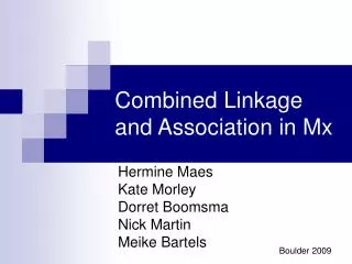
5. Genotypic similarity between relatives IBDAlleles shared Identical By Descent are a copy of the same ancestor allele Pairs of siblings may share 0, 1 or 2 alleles IBD The probability of a pair of relatives being IBD is known as pi-hat M3 M1 M2 M3 Q3 Q1 Q2 Q4 M1 M2 M3 M3 Q1 Q2 Q3 Q4 IBS IBD M1 M3 M1 M3 2 1 Q1 Q4 Q1 Q3

6. MZ=1.0 DZ=0.5 MZ & DZ = 1.0 1 1 1 1 1 1 1 1 Q A C E E C A Q e c a q q a c e PTwin1 PTwin2

7. Distribution of pi-hat • Adult Dutch DZ pairs: distribution of pi-hat at 65 cM on chromosome 19 • Model resemblance (e.g. correlations, covariances) between sib pairs, or DZ twins, as a function of DNA marker sharing at a particular chromosomal location

8. DZ by IBD status Variance = Q + F + E Covariance = πQ + F + E

9. Covariance Statements G2: DZ IBD2 twins Matrix K 1 Covariance F+Q+E | F+K@Q _ F+K@Q | F+Q+E; G3: DZ IBD1 twins Matrix K .5 Covariance F+Q+E | F+K@Q _ F+K@Q | F+Q+E; G4: DZ IBD0 twins Covariance F+Q+E | F_ F | F+Q+E;

10. DZ by IBD status + MZ

11. Covariance Statements +MZ G2: DZ IBD2 twins Matrix K 1 Covariance A+C+Q+E | H@A+C+K@Q _ H@A+C+K@Q | A+C+Q+E; G3: DZ IBD1 twins Matrix K .5 Covariance A+C+Q+E | H@A+C+K@Q _ H@A+C+K@Q | A+C+Q+E; G4: DZ IBD0 twins Covariance A+C+Q+E | H@A+C_ H@A+C | A+C+Q+E; G5: MZ twins Covariance A+C+Q+E | A+C+Q _ A+C+Q | A+C+Q+E;

12. Using the full distribution • More power if we use all the available information • So instead of dividing the sample we will use as a continuous coefficient that will vary between sib-pair across loci

13. DZ twins using full distribution of pihat Covariance F+E+Q | F+P@Q_ F+P@Q | F+E+Q ; DZ=1 1 1 1 1 1 1 Q F E E F Q e f q q f e PTwin1 PTwin2

14. The example data Lipid data: apoB

15. !script for univariate linkage - pihat approach !DZ/SIB #loop $i 1 4 1 #define nvar 1 #NGroups 1 DZ / sib TWINS genotyped Data NInput=324 Missing =-1.0000 Rectangular File=lipidall.dat Labels sample fam ldl1 apob1 ldl2 apob2 … Select apob1 apob2 ibd0m$i ibd1m$i ibd2m$i ; Definition_variables ibd0m$i ibd1m$i ibd2m$i ; Pihat.mx This use of the loop command allows you to run the same script over and over moving along the chromosome The format of the command is: #loop variable start end increment So…#loop $i 1 4 1 Starts at marker 1 goes to marker 4 and runs each locus in turn Each occurrence of $i within the script will be replaced by the current number ie on the second run $i will become 2 With the loop command the last end statement becomes an exit statement and the script ends with #end loop

16. !script for univariate linkage - pihat approach !DZ/SIB #loop $i 1 4 1 #define nvar 1 #NGroups 1 DZ / sib TWINS genotyped Data NInput=324 Missing =-1.0000 Rectangular File=lipidall.dat Labels sample fam ldl1 apob1 ldl2 apob2 … Select apob1 apob2 ibd0m$i ibd1m$i ibd2m$i ; Definition_variables ibd0m$i ibd1m$i ibd2m$i ; Pihat.mx This use of the ‘definition variables’ command allows you to specify which of the selected variables will be used as covariates The value of the covariate displayed in the mxo will be the values for the last case read

17. !script for univariate linkage - pihat approach !DZ/SIB #loop $i 1 2 1 #define nvar 1 #NGroups 1 DZ / sib TWINS genotyped Data NInput=324 Missing =-1.0000 Rectangular File=lipidall.dat Labels sample fam ldl1 apob1 ldl2 apob2 … Select apob1 apob2 ibd0m$i ibd1m$i ibd2m$i ; Definition_variables ibd0m$i ibd1m$i ibd2m$i ; Begin Matrices; X Lower nvar nvar free ! residual familial F Z Lower nvar nvar free ! unshared environment E L Full nvar 1 free ! qtl effect Q G Full 1 nvar free ! grand means H Full 1 1 ! scalar, .5 K Full 3 1 ! IBD probabilities (from Merlin) J Full 1 3 ! coefficients 0.5,1 for pihat End Matrices; Specify K ibd0m$i ibd1m$i ibd2m$i Matrix H .5 Matrix J 0 .5 1 Start .1 X 1 1 1 Start .1 L 1 1 1 Start .1 Z 1 1 1 Start .5 G 1 1 1 Pihat.mx

18. Begin Algebra; F= X*X'; ! residual familial variance E= Z*Z'; ! unique environmental variance Q= L*L'; ! variance due to QTL V= F+Q+E; ! total variance T= F|Q|E; ! parameters in one matrix S= F%V| Q%V| E%V; ! standardized variance component estimates P= ???? ; ! estimate of pihat End Algebra; Labels Row S standest Labels Col S f^2 q^2 e^2 Labels Row T unstandest Labels Col T f^2 q^2 e^2 Means G| G ; Covariance F+E+Q | F+P@Q_ F+P@Q | F+E+Q ; Option NDecimals=4 Option RSiduals Option Multiple Issat !End !test significance of QTL effect ! Drop L 1 1 1 Exit #end loop Pihat.mx You need to fix this before you run the script

19. Run the script across your region and add the -2LL to the xls file

20. Converting chi-squares to LOD scores • For univariate linkage analysis (where you have 1 QTL estimate) Χ2/4.6 = LOD

21. Converting chi-squares to p values • Complicated • Distribution of genotypes and phenotypes • Boundary problems • For univariate linkage analysis (where you have 1 QTL estimate) p(linkage)=

23. What does it mean?

24. Alternative approach • is a summary statistic • Convenient • Loss of information • .5 can mean p.ibd0=0 p.ibd1=1 p.ibd2=0 or p.ibd0=.2 p.ibd1=.6 p.ibd2=.2 • Use all the information

25. Alternative approach • Model each of the possible outcomes • IBD0 IBD1 IBD2 • Weight each of the models by the probability that it is the correct model • The pairwise likelihood is equal to the sum of likelihood for each model multiplied by the probability it is the correct model • The combined likelihood is equal to the sum of all the pairwise likelihoods

26. DZ pairs * pIBD2 + * pIBD1 + * pIBD0

27. How to do this in mx? Tells Mx we will be using 3 different means and variance models • Script mixture.mx DZ / sib TWINS genotyped Data NInput=324 NModel=3 Missing =-1.0000 Rectangular File=lipidall.dat Labels …. Select apob1 apob2 ibd0m$i ibd1m$i ibd2m$i ; Definition_variables ibd0m$i ibd1m$i ibd2m$i ;

28. How to do this in mx? This script runs an FQE model L is the QTL VC path coefficent Begin Matrices; X Lower nvar nvar free ! residual familial F Z Lower nvar nvar free ! unshared environment E L Full nvar 1 free ! qtl effect Q G Full 1 nvar free ! grand means H Full 1 1 ! scalar, .5 K Full 3 1 ! IBD probabilities (from Merlin) U Unit 3 1 … Matrix H 0.5 Specify K ibd0m$i ibd1m$i ibd2m$i We are placing the prob. Of being IBD 0 1 & 2 in the K matrix

29. How to do this in mx? Begin Algebra; F= X*X'; ! residual familial variance E= Z*Z'; ! unique environmental variance Q= L*L'; ! variance due to QTL V= F+Q+E; ! total variance

30. How to do this in mx? Means U@G| U@G; Covariance F+Q+E | F _ F | F+Q+E _ ! IBD 0 Covariance matrix F+Q+E | F+H@Q _ F+H@Q | F+Q+E _ ! IBD 1 Covariance matrix F+Q+E | F+Q _ F+Q | F+Q+E; ! IBD 2 Covariance matrix Weights B ; The means matrix contains corrections for age and sex – it is repeated 3 times and vertically stacked Tells Mx to weight each of the means and var/cov matrices by the IBD prob. which we placed in the B matrix

31. Your job • Pick a number location that you ran with the pihat script • Change the script to run linkage at the location you picked • Test for linkage

33. Summary • Weighted likelihood approach more powerful than pi-hat • Quickly becomes unfeasible • 3 models for sibship size 2 • 27 models for sibship size 4 • Q: How many models for sibship size 3? • For larger sib-ships/arbitrary pedigrees pi-hat approach is method of choice

34. Break – and then association

35. Association Introduction

36. Association • Simplest design possible Correlate phenotype with genotype

37. The equivalent for a quantitative trait- run a regression Yi = a + bXi + ei where Yi = trait value for individual i Xi = 1 if allele individual i has allele ‘A’ 0 otherwise i.e., test of mean differences between ‘A’ and ‘not-A’ individuals Play with Association.xls 0 1

38. 2a Genotype Genetic Value BB Bb bb a d -a Biometrical model d bb midpoint Bb BB Va (QTL) = 2pqa2 (no dominance)

39. How can we do this in Mx?

40. Where this goes wrong… • Chose a phenotype – chopstick use • Collect 2 groups - cases and controls • Unrelated individuals – university students • Matched for relevant covariates – age sex 0 1

41. Where this goes wrong… • Pick your candidate gene and type it – SUSHI (Successful use of selected hand instruments gene) • Count the number of cases and controls with each genotype – highly significant and replicatable 0 1

42. Obviously this is a spurious example • The cases were of Asian decent, the controls were of Caucasian decent • SUSHI – was a histocompatability antigen gene with different allele frequencies in different racial groups • This confound is known as population stratification (Yes this is a fairy tale but it is based on a real asthma study)

43. Practical – Find a gene for sensation seeking: • Two populations (A & B) of 100 individuals in which sensation seeking was measured • In population A, gene X (alleles 1 & 2) does not influence sensation seeking • In population B, gene X (alleles 1 & 2) does not influence sensation seeking • Mean sensation seeking score of population A is 90 • Mean sensation seeking score of population B is 110 • Frequencies of allele 1 & 2 in population A are .1 & .9 • Frequencies of allele 1 & 2 in population B are .5 & .5

44. .01 .18 .81 .25 .50 .25 Genotypic freq. Sensation seeking score is the same across genotypes, within each population. Population B scores higher than population A Differences in genotypic frequencies

45. Suppose we are unaware of these two populations and have measured 200 individuals and typed gene X The mean sensation seeking score of this mixed population is 100 What are our observed genotypic frequencies and means?

46. Calculating genotypic frequencies in the mixed population Genotype 11: 1 individual from population A, 25 individuals from population B on a total of 200 individuals: (1+25)/200=.13 Genotype 12: (18+50)/200=.34 Genotype 22: (81+25)/200=.53

47. Calculating genotypic means in the mixed population Genotype 11: 1 individual from population A with a mean of 90, 25 individuals from population B with a mean of 110 = ((1*90) + (25*110))/26 =109.2 Genotype 12: ((18*90) + (50*110))/68 = 104.7 Genotype 22: ((81*90) + (25*110))/106 = 94.7

48. Genotypic freq. .13 .34 .53 Gene X is the gene for sensation seeking! Now, allele 1 is associated with higher sensation seeking scores, while in both populations A and B, the gene was not associated with sensation seeking scores… FALSE ASSOCIATION

49. Dm = Difference in subpopulation mean =-10 5 Overestimation 4 =-5 3 Genuine allelic effect=+2 2 Estimated value of allelic effect Underestimation 1 0 =5 -1 Reversal effects -2 =10 -3 0.49 0.42 0.35 0.28 0.07 0.00 -0.07 -0.28 -0.35 -0.42 -0.49 0.21 0.14 -0.14 -0.21 Differencein gene frequency in subpopulations False positives and false negatives Posthuma et al., Behav Genet, 2004

50. How to avoid spurious association? True association is detected in people coming from the same genetic stratum • Can check that individuals come from the same population using a large set of highly polymorphic genes – genomic control • Can use family members as controls – family based association