ECE 636 Reconfigurable Computing Lecture 5 FPGA Routing
350 likes | 581 Views
ECE 636 Reconfigurable Computing Lecture 5 FPGA Routing. Overview. Routability Estimation 1 step routing 2 step routing Pathfinder (and Pathfinder derivatives). Island-Style Devices. Two dimensional problem (X+Y)!/(X!Y!) possible paths Restricted within bounding box. FPGA issues.

ECE 636 Reconfigurable Computing Lecture 5 FPGA Routing
E N D
Presentation Transcript
Overview • Routability Estimation • 1 step routing • 2 step routing • Pathfinder (and Pathfinder derivatives)
Island-Style Devices • Two dimensional problem • (X+Y)!/(X!Y!) possible paths • Restricted within bounding box
FPGA issues • Often want a fast answer. May be willing to accept lower quality result for less place/route time. • May be interested in knowing wirability without needing the final configuration. • Fast placement: constructive placement, iterative improvement through simulated annealing.
Maze routing • Will find shortest path for a single wire, if such a path exists. • Two phases: • Label nodes with distance, radiating from source. • Use distances to trace from sink to source, choosing a path that always decreases distance to source.
L S L C Maze Routing • Evaluate shortest feasible paths based on a cost function • Like row-based device global route allocates channel bandwidth not specific solutions. • Formulate cost function as needed to address desired goal.
Two main type of FPGA routers • Two phase routers • Global router assigns net connections to specific FPGA channels • Detailed router “expands” choices in channel to select available wires • One phase routers • Channel assignment and wire selection happens in one routing pass • Two phase routers were initially popular • Simpler to write and faster to execute • More closely models ASIC routing techniques • One phase routers shown to give MUCH better performance
L L L L L L 1 1 1 2 2 2 3 3 3 L L L L L L Connection B Connection C Connection A Consider This Example • Limited resources cause dependencies • Need to enumerate possible routes • Prioritize based on cost factors.
2,2 L 2,3 C 3,3 S 1 1 C 3,4 1 1 L 4,4 Graph Expansion • Enumerate possible expansions • Limited by switchbox and connection box. 1 1 1 1 1 1
Detailed graph expansion • Consider all possible routes within selected channels • Limited by connection block and switch block connectivity
Detailed Routing: Lemieux and Brown • Issues to consider • Some wires span multiple blocks • Need to allocate long connections to long wires • Step 1: • For each connection, locate all possible routes • Step 2: • Use complicated cost function to route connections • Many limitations • No seamless way to deal with nets with high fanout • What happens if we run out of tracks? • Doesn’t support multiple iterations.
Weighting Graph Costs • Select paths that have fewest negative effects on others. • Identify paths that are essential for a connection. • Sharing factor to enhance high-fanout • Selecting longer segments for nets to reduce wire delay • Weighting these factors is not an easy task
VPR: One-step FPGA Router • Combined global and detailed routing together • Uses “expansion wavefront” starting at net source • Expansion performed based on node cost
Routing Tradeoffs • Bias router to find first, best route. • Vary number of node expansions using: pcosti = (1 – a) x pcosti-1 + ncosti + a x disti
VPR versus Sega • VPR allows full search of implementation space. • Effective for multi-fanout nets • 40% better than Sega
Making One-Step Routing Faster • How should net fanouts be orders? • Does this reduce area? • What is the effect on performance? • Relatively straightforward algorithm
Making One-Step Routing Faster • What happens to the expansion list if there are many sinks? • Binning helps speed up router run time. • Many high fanout nets now handled by special global routing network.
Dealing with Multi-Fanout Nets • Difficult to estimate routing area associated with multi-fanout nets • Need to modify cost estimation
Dealing with Multi-Fanout Nets • Use the cost factor to help scale bounding box costs associated with placement and routing estimation • Very useful in determining likely routing success
Dealing with Multi-Fanout Nets • Routing becomes much easier as the amount of routing resources increases
Linear growth of routing time? • In the absence of congestion, the routing problem becomes greedy • In general wiring should increase at a more than linear rate with circuit size • Greedy allocation of resources may obscure this.
Routing Estimation for Island-style Devices • Develop approach to use wire length to determine routability of device. • Westimate = total wirelength/2*Nblocks* U • Difficult to determine U, dependent on Fc and Fs • Real difficulty in evaluating “wire length”
Estimating Wirelength • Multi-fanout nets present a challenge. • Use cost correction factor to adjust bounding box value (e.g. F=4, C=1.08) • Not clear what to do for timing driven • 84% accuracy for 15 benchmarks (Rose/Swartz) • Even works for segmented devices.
Track count estimation • Use to determine if device will route successfully • Less of an issue for today’s commercial FPGAs • Not really helpful for timing-driven compilation
Architectural Limitation • Routing architecture necessitates domain selection. • Bigger effect for multi-fanout nets
Domain Negotiation • Evaluate occupancy of domains adjacent to outputs prior to net routing • Rank domains by routability • Penalize domains with little or no likelihood of successful completion. • Add domain rank to node cost function at net output. pcosti = (1 – a) x pcosti-1 + ncosti + a x disti + rd
Results: Fast Routing – FFT16 • Domain negotiation has larger effect as track width is reduced.
Routing Results Summary • Low-stress case shows order of magnitude speedup • Routing proportional to wire length • Domain negotiation reduces difficult route time by a factor of 2.
Difficult Routing Case Results • Depth-first case needs same track count as minimum breadth-first track count.
Pathfinder • Use a non-decreasing history value to represent congestion. • Similarities to multi-commodity flow • Can be implemented efficiently but does require substantial run time • Only update after an interation. ci = (1 + hn * hfac) * (1 + pn * pfac) + bn, n-1
Timing-Driven Routing • Add delay cost component to routing. • Represent delay along path as RC chain. Buffering important here. • Note that timing driven routing selects most distant point for first route. • Sets upper bound on delay. • Need for combined breadth-first congestion and timing-driven route.
Timing-Driven Routing • Difficult to estimate remaining timing along a path • Difficult to balance costs for each critical net • Some routers attempt to “look-ahead” to anticipate congested or time-critical areas • Optimal approaches have generally failed.
Combined Placement and Routing • Used depth-first route to select initial connections • Swap blocks and rip up attached nets • Bias nets that span the bulk of device onto long-line resources. • Took 16X longer than place and route • 8% to 15% improvement.
Summary • Routing a difficult problem based on device size, complexity • Early 2-step approaches became obsolete as device sizes grew. • Pathfinder extensively used to determine best, shortest paths. • Most routers are highly advanced.