ICS 214B: Transaction Processing and Distributed Data Management
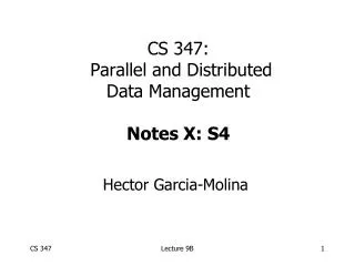
ICS 214B: Transaction Processing and Distributed Data Management. Lecture 10: Distributed Query Optimization Professor Chen Li. Optimization Process Overview. Generate query plans Estimate size of intermediate results Estimate cost of plan ($,time,…). P 2. P 3. P n. P 1.

ICS 214B: Transaction Processing and Distributed Data Management
E N D
Presentation Transcript
ICS 214B: Transaction Processing and Distributed Data Management Lecture 10: Distributed Query Optimization Professor Chen Li
Optimization Process Overview Generate query plans Estimate size of intermediate results Estimate cost of plan ($,time,…) P2 P3 Pn P1 C1 C2 C3 Cn pick minimum Notes 10
Query Plans • Space of query plans is much larger than in centralized db • More ways to implement relational operators (joins, sorts, aggregates) • Possibility for inter-operator parallelism Notes 10
Distributed Query Optimization • Tricks for relational operators • Sorting • Joins • Aggregates • Select • Tricks for inter-operations parallelism • Strategies for optimization Notes 10
Parallel/distributed sort Input: • (a) relation R on single site/disk; or • (b) R fragmented/partitioned by sort attribute; or • (c) R fragmented/partitioned by other attribute. Notes 10
Output (a) sorted R on single site/disk or (b) fragments/partitions sorted F1 F2 F3 19 ... 5 ... 12 ... 20 6 ... 15 21 10 50 Notes 10
Basic sort • R(K,…), sort on K • Fragmented on K Vector: k0, k1, … kn k0 k1 7 11 27 10 20 3 17 22 14 Notes 10
Algorithm: each fragment sorted independently • If necessary, ship results Notes 10
Range partitioning sort • R(K,….), sort on K • R located at one or more site/disk,not fragmented on K Notes 10
Algorithm: (a) Range partition on K (b) Basic sort Ra Rb Local sort R1 R’1 ko Result Local sort R’2 R2 k1 Local sort R3 R’3 Notes 10
Selecting a good partition vector Ra Rb Rc 7 ... 31 ... 10 ... 52 8 12 11 15 4 14 11 32 17 Notes 10
Example • Each site sends to coordinator: • Min sort key • Max sort key • Number of tuples • Coordinator computes vector and distributes to sites (also decides # of sites for local sorts) Notes 10
Expected tuples: 5 10 15 20 k0? 2 1 [assuming we want tosort at 2 sites] Sample scenario: Coordinator receives: SA: Min=5 Max=10 # = 10 tuples SB: Min=7 Max=17 # = 10 tuples Notes 10
Expected tuples: 5 10 15 20 k0? 2 1 [assuming we want tosort at 2 sites] Expected tuples = Total tuples with key < ko 2 2(ko - 5) + (ko - 7) = 10 3ko = 10 + 10 + 7 = 27 ko = 9 Notes 10
Variations • Send more info to coordinator • Partition vector for local site Eg. Sa: 3 3 3 # tuples 5 6 8 10 local vector - Histogram 5 6 7 8 9 10 Notes 10
More than one round E.g.: (1) Sites send range and # tuples (2) Coordinator returns “preliminary” vector Vo (3) Sites tell coordinator how many tuples in each Vo range (4) Coordinator computes final vector Vf Notes 10
Parallel external sort-merge Ra Rb • Same as range-partition sort, except sort first Local sort Ra’ R1 ko Result Rb’ Local sort R2 k1 In order R3 Merge Notes 10
Distributed Query Optimization • Overview • Tricks for relational operators • Sorting • Joins • Aggregates • Select • Tricks for inter-operations parallelism • Strategies for optimization Notes 10
Parallel/distributed Join Input: Relations R, S May or may not be partitioned Output: R S Result at one or more sites Notes 10
A S1 R1 S2 R2 S3 R3 Partitioned Join (Equi-join) R S Local join R S f(A) Result f(A) Notes 10
Local join A R1 Sa S1 R2 S2 Sb f(A) Result f(A) S3 R3 Sc Partitioned Join (Equi-join)R S Ra Rb Notes 10
Notes: • Same partition function f is used for both R and S (applied to join attribute) • f can be range or hash partitioning • Local join can be of any type (use any ICS214A optimization) • Various scheduling options e.g., (a) partition R; partition S; join (b) partition R; build local hash table for R; partition S and join Notes 10
Even more notes: • Selecting good partition function f very important: • Number of fragments • Hash function • Partition vector • Good partition vector • Goal: | Ri |+| Si | the same • Can use coordinator to select Notes 10
S R1 S R2 S R3 Asymmetric fragment + replicate join Local join Ra Sa Rb Sb f partition Result union Notes 10
Notes: • Can use any partition function f for R (even round robin) • Can do any join — not just equi-join e.g.: R S R.A < S.B Notes 10
R2 S2 S is partitioned in similar fashion into m fragments R1 S1 R1 S2 Result R2 S1 All nxm pairings of R,S fragments R3 S1 R3 S2 Notes 10
A A A A A A A A Semijoin Reducers • Goal: reduce communication traffic • R S (R S) S or R (S R) or (R S) (S R) Notes 10
Ans: R S AR = [2,10,25,30] A C 10 y 25 w S R = Example: R S A B A C R S 2 a 3 x 10 b 10 y 25 c 15 z 30 d 25 w 32 x Notes 10
better if say |B| is large 2 a 3 x 10 b 10 y A B A C R S 25 c 15 z 30 d 25 w 32 x • Computing transmitted data in example: • with semi-join R (S R): • T = 4 |A| +2 |A+C| + result • with join R S: • T = 4 |A+B| + result Notes 10
A A A A In general: • Say R is smaller relation • (R S) S better than R S if size (A S) + size (R S) < size (R) • Similar comparisons for other semi-joins • Remember: only taking into account transmission cost Notes 10
Trick: Encode A S (or A R ) as a bit vector key in S <----one bit/possible key-------> 0 0 1 1 0 1 0 0 0 0 1 0 1 0 0 Notes 10
Option 1: R’ S’ T where R’ = R S; S’ = S T Option 2: R’’ S’ T where R’’ = R S’; S’ = S T Three-way joins with semi-joins Goal: R S T • Many options! • Number of semi-join options is exponential in # of relations in join Notes 10
Distributed Query Optimization • Tricks for relational operators • Sorting • Joins • Aggregates • Select • Tricks for inter-operations parallelism • Strategies for optimization Notes 10
Aggregates • Aggregates • Partition by grouping attributes; compute aggregate locally Notes 10
sum sum Example: Ra Rb • sum (sal) group by dept Notes 10
sum sum sum sum less data! Example: Ra Rb • sum (sal) group by dept Notes 10
Enhancements for aggregates • Perform aggregate during partition to reduce data transmitted Notes 10
Distributed Query Optimization • Tricks for relational operators • Sorting • Joins • Aggregates • Select • Tricks for inter-operations parallelism • Strategies for optimization Notes 10
Selection • Range or hash partition • Straightforward But what about indexes? Notes 10
Indexing • Can think of partition vector as root of distributed index: ko k1 Local indexes Site 1 Site 2 Site 3 Notes 10
Index on non-partition attribute Index sites Tuple sites ko k1 Notes 10
Summary: Query processing • Decomposition and Localization • Optimization • Overview • Tricks for joins, sort,.. • Tricks for inter-operations parallelism • Strategies for optimization Notes 10
Inter-operation parallelism • Pipelined • Independent Notes 10
Pipelined parallelism Site 2 c Site 1 S R result Site 1 Join Probe Tuples matching c R S Notes 10
Independent parallelism R S T V (1) temp1 R S; temp2 T V (2) result temp1 temp2 Site 2 Site 1 Notes 10
Summary: Query processing • Decomposition and Localization • Optimization • Overview • Tricks for joins, sort,.. • Tricks for inter-operations parallelism • Strategies for optimization Notes 10
Query optimization • Cost estimation • Strategies for exploring plans Q min Notes 10
Cost estimation • In centralized db, estimating size of intermediate results is important to evaluate cost of plan • True for distributed query processing • Same techniques (from ICS214) • In centralized db, cost of query plan = number of IOs • Not necessarily true for distributed query processing Notes 10
In distributed db: # IOs may not be best metric e.g., Transmission time may dominate work work answer at site at site T1 T2 >>>---------TIME---------> or $ Notes 10
Another reason why plain IOs not enough:Parallelism Plan APlan B site 1 50 IOs 100 IOs site 2 70 IOs site 3 50 IOs Notes 10