Download

1 / 67
670 likes | 800 Views
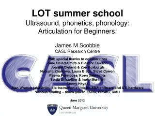
LOT summer school Ultrasound, phonetics, phonology: Articulation for Beginners!. With special thanks to collaborators Jane Stuart-Smith & Eleanor Lawson Joanne Cleland & Zoe Roxburgh Natasha Zharkova , Laura Black, Steve Cowen Reenu Punnoose , Koen Sebreghts

E N D
LOT summer schoolUltrasound, phonetics, phonology: Articulation for Beginners! With special thanks to collaborators Jane Stuart-Smith & Eleanor Lawson Joanne Cleland & Zoe Roxburgh Natasha Zharkova, Laura Black, Steve Cowen ReenuPunnoose, KoenSebreghts Sonja Schaeffler & Ineke Mennen ConnyHeyde Alan Wrench (aka Articulate Instruments Ltd) for AAA software and UTI hardware Various funding – thank you to ESRC, EPSRC, QMU June 2013 James M Scobbie CASL Research Centre
Introduction to articulation • Brief overview of techniques • Ultrasound tongue imaging • Playtime • Technical issues and the nitty gritty of data • Maybe a linguistic illustration • Malayalam liquids Structure
Different laboratories have different solutions • Exemplification will be based around current practice at QMU / Articulate Instruments Ltd • Topics (mostly in this order) • Resolution, fixed aspect ratio representations • Up, down and horizontal…the bite plane • Quick averaging multiple tongue surfaces • Statistical testing of difference between averages • Two tongues, synching, de-interfacing • Video-rate vs. (ultra) high speed ultrasound Technical issues
More echo-pulse beams / scanlines means more resolution in a circumferential direction • Let’s assume 1 scanline each 2° (180 in a circle) • Scanlines get further apart the further they are from the probe • At 90mm from probe centre, resolution is 3.14mm • At 60mm, resolution is 2mm • 45mm it is 1.6mm • To maintain these resolutions… • A 90° field of view would need 46 scanlines • A 135° field of view would need 69 scanlines Spatial resolution around the curve
More sample points means more resolution in a radial direction • 8cm depth with 256 sample points = 0.3mm/point • Assuming enough pixels to represent each point Spatial resolution along the radii
The fan shape is presented on a rectangular screen, and occupies a proportion of that space • A TV image has a certain number of data points horizontal / vertical (e.g. in NTSC) • These are digitised into pixels at a given resolution… • Horizonatal in the head is not the same thing as being parallel to the x-axis in the rectangle! Rectangular images
Approximate location of EMA coils in analysis of /u/ fronting in SSBE Harrington, Kleber & Reubold 2011
Approximate location of EMA coils in analysis of /u/ fronting in SSBE – 2-4mm back/below /i/ Harrington et al
Example of a UTI vowel space, rotated to occlusal bite plane, with average curves (± 1sd) • Left pane is standard view, right the UTI view… UTI single SSE speaker
Use a “bite plate” to detect the unique occlusal plane for each speaker, as in typical in EMA • Flat plane defined on upper dentition surface • Also provides common origin as well as axes • Scobbie, Lawson, Cowen, Cleland & Wrench (2012) ms. – I might be able to put this online… Finding the “horizontal”
In humans, the directions "rostral" and "caudal" often become confused with anterior and posterior, or superior and inferior. The difference between the two is most easily visualized when looking at the head, as can be seen in the image to the right. From the most caudal of positions in the nervous system (of a person) to a nearby, rostral area, it is equally accurate to say the area in question is rostral as to say it is superior. However, in the frontal lobes of the telencephalon, to say an area is rostral to a nearby area is equivalent to saying it is anterior. Those two lines lie on planes perpendicular to one another. This occurs, as becomes clear in the diagram, due to the intuitive yet curious curving "C" shape of rostrocaudal directionality when discussing the human brain. wikipedia
bite plate Occlusalbiteplane trace
Six young adult female speakers • Varying slopes (mean 18.5°) • Varying vertical offset • Varyinghorizontal offset back of plate Variation in bite plane
Mean hard palate trace (black) and biteplane trace grey), automatic curve fitting Overlay of 6 hard palates
Normalised (translation and rotation) to rear of bite plane and relocation of origin (+45mm) • Better palate trace alignment, with one “rogue” Palates normalised to bite planes
Palates can be used to orientate between sessions, by swallowing (e.g. water or yoghurt) • Longitudinal, within-speaker • Just line up the palates! • Easy, huh?! • Cross-speaker • Might be better than bite plate when worrying about close approximation constrictions • Bite plate might be better for open approximation • The probe can be moved instead • A consistent articulation can be used, eg [u] Alternatives
MRI data is collected supine – does it matter? • Upright L and supine R “pop” vowel • Wrench et al 2011 Upright / supine
6 female speakers, varied accents • 5 reps of pep and of pop in randomised list of vowels • 4 blocks, repeating upright/supine set twice • Upright first for 3, supine first for 3 • Pharyngeal slump under gravity of about 3mm • And a couple of cases of blade raising Summary
Averaging along 42 fan-grid radii, “parallel” to scan-lines / echo-pulse beam from the probe Averaging within AAA
n tokens along radius r Tokens of [s] from /si/
vs. a different condition Tokens of [s] from /sa/ and /si/
t-test of the difference between mean tongue contour at crossing point at each fan line • 2-tailed test assuming unequal variances and unequal sample sizes • No Bonferroni or other corrections • Up to 5 or 6 adjacent radii, mean distance from probe is correlated, perhaps indicating non-independence of such “close” measures • For a linguistic interpretation of difference, 5 or 6 adjacent radii, all at p<0.05 on t-test is more important than p<0.0001 on one radius 2 groups of curves
2 speakers, 4 frames each • 42 radii per speaker… • What % of correlations between two random radii are significant, depending on the distance between them • Radial distance • Grand mean • All parts of tongue pooled • More cases of adjacent than longdistancecomparisons Pilot correlation v1
A range of 9 varied tongue shapes (9 single frames) from each speaker • 4 samples for each frame – roughly equally spaced • Is there a correlation for fans 10 apart? • 9? 8? 7? … • Pilot B (NI1) Pilot correlation v2
3 attempts – more long-distance significance found • One sectoron the fan is 7fanlines
Just two sample points per frame, front and back? • Pilot 2 A = 9 fans rather than 8 were significant (n=18 observations, so lower values of r were significant) • Or one in the middlelooking forwards and backwards? • Or use many more target types? • Or ones that show more subtle differences, such as a set of CV transitions, including every frame, not just varied targets What to try next?
Raw tongue curves again Tokens of [s] from /sa/ and /si/
Significant root advancement (~5mm) and palatalisation (~4mm) in /si/ • More than 5 adjacent fans where p<0.05, but in 2 areas Mean /sa/ vs. /si/
SS-ANOVA best fit lines (∓ 95% c.i.) - Davidson Mean /sa/ vs. /si/
Exploring treating >5 fan lines at p<0.05 as categorically “significant” but quantifying it all: • Including crossing/pivot points • Ignore significance if curves are low confidence • Quantify length of the significant tongue surface • Estimate total difference in area Mean /sa/ vs. /si/
Thick lines for means – cf overlap, non overlap, and crossings Single speaker (SSE) Neutral space
Wrench & Scobbie (2006) list some of the problems with video-ultrasound resulting from buffering multiple probe scans into one image • More than one scan from the probe in an image • Partial scans from the probe in an image • Don’t forget 30fps is about 33ms, so synch is vague • Some solutions, • Use raw probe data (cine loop) but this costs € • Use a high scan rate (more than twice NTSC) and then deinterlace the video to 60fps • Halves vertical spatial resolution (rectangular up) The two tongue problem
The scanner scans and makes screen images Video digital capture & buffering
The scanner scans and makes screen images Video digital capture & buffering
In these images, two apparent tongues show the effect of two scans in the same buffer, on odd and even video “lines” Plain 30fps video
Deinterlace video images to 30fps (16ms or so) • “Cineloop” digital output can be stored locally on US scanners • Full rectangular cine images • Approx 15 second chunks • Continuous audio recordings need post-processing alignment • AAA / QM Ultrasonix-based system • Data stored as raw probe echo-pulse returns • Synchronised at source with audio at each frame • Video channel freed up, and can be used to capture lip videos Solutions
76 scan lines, 100fps, FoV 112° High speed
39 scan lines, 196fps, FoV 112° Ultra-high speed
25 scan lines, 306fps, FoV 112° Ultra-high speed
g ɔ d back front time “dog” – ultra high speed 382fps
hs-UTI @ 382fps & video @ 60fps, 300ms • Constriction-tracking, comparable to but different to flesh-point tracking “tongue blade height” during [d]
Video demo, deinterlaced lip camera 60fps [folder] • UTI old dutch and labialised english r [link] • Lip ultrax kids [link] – deinterlaced ring [link] • High speed UTI 100fps • Malayalam retroflex lateral [folder] • Slomo [link] • Slomo with spline [link] • Real speed with spline [link] Demo videos
Two darker (tongue root) liquids, L /ɭ/and R /r/ • Three clearer (ATR, ~pal’ised) l /l/, r /ɾ/, 5 zh Single frame targets
Malayalam trill /r/ R between /a/ • Left = closing half of gesture • Right = opening half • Note trill motion in blade and stable root High speed (100fps)
Malayalam tap /ɾ/ between /a/ • Note greater movement in root, pivot point High speed (100fps)
Malayalam retroflex flap /ɭ/ • Stable root, mobile blade, slower approach with very fast release (nb some UTI artefacts) of over 400mm/sec peak velocity High speed (100fps)