Download
1 / 37
370 likes | 423 Views
Learn about mass transfer, Fick's law, and convective mass transfer processes with chemical reactions. Explore unsteady diffusion and axial dispersion models in MHMT14. Understand the analogies with heat transfer and the principles of penetration depth in transient convective diffusion problems, like RTD - axial dispersion. Get insights into molar flux, molar velocity, and mass transfer phenomena in mixtures through detailed examples and correlations.

E N D
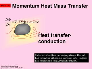
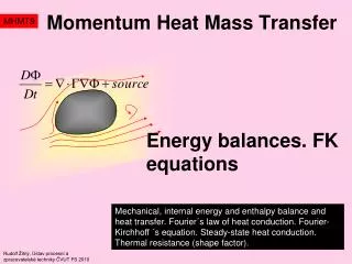
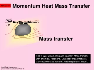
Momentum Heat Mass Transfer MHMT14 Mass transfer Fick´s law. Molecular mass transfer. Mass transfer with chemical reactions. Unsteady mass transfer. Convective mass transfer. Axial dispersion model. Rudolf Žitný, Ústav procesní a zpracovatelské techniky ČVUT FS 2010
Mass Transfer - diffusion MHMT14 General transport equation for property P can be applied for the mass transport too In case of mixture of several components (we shall consider as an example binary mixture consisting in components A and B) the transported properties P are mass concentrations A of components proportional to mass fraction A and density Remark: components can be for example water vapour and air, or chemical species, CH4, O2, N2,… Mass flux of a component A is directly proportional to the driving potential – gradient of concentration (or mass fraction), this is Fick’s law
Mass Transfer – transport eqs. MHMT14 Substituting into the general transport equation we obtain transport equations for each component separately Using identity it is possible to write the transport equation as
Mass Transfer – transport eqs. MHMT14 So far everything seems to be as usual. For example exactly the same equation (Fourier Kirchhoff) holds if you substitute T for the mass fraction A. However, what does it mean the velocity u in the case of mixture? Individual components are moving with different velocities and resulting mass flux (kg/(m2.s)) is the sum of the component fluxes Especially at gases the concentrations are expressed in terms of molar concentrations and molar fractions
1D – steady diffusion A1 yA1 A2 yA2 z L MHMT14 General transport equation for steady state, constant density and DAB, without source term reduces to For gases it is more suitable to assume constant overall pressure and to use molar fractions (yA) instead mass fractions
1D – steady diffusion yA2 z yA(z) L yA1 yA2 L yA(z) z yA1 MHMT14 Let us consider the case that u(m)=0, i.e. the same number of molecules A is moving in one direction as the number of B molecules in the opposite direction. This is so called equimolar diffusion and concentration profile is linear Different case is for example evaporation of water vapors (component A) into air (component B). Air cannot be absorbed in water and therefore mass or molar flux is zero (uB=0) and mean molar velocity is determined by the velocity of vapors uA (how to calculate the molar flux NzA will be shown in the next slide) Equation of transport (steady state, without sources and unidirectional diffusion)
1D – steady diffusion MHMT14 The mean molar velocity (convective velocity) for uB=0 and the resulting molar flux NA follow from the definition of molar flux and the Fick´s law Substituting for yA the previously calculated exponential yAprofile gives and the molar fraction profile … and you see that this profile is also independent of DAB
Analogy heat and mass transfer MHMT14 We could continue the lecture by unsteady diffusion, in a similar way and with similar results as in the heat transfer. For example the principle of penetration depth remains and thus it is possible to estimate the range of concentration changes corresponding to duration of a concentration disturbance (typical problem: calculate the depth of soil filled by petrol spilled on surface at a specified time after accident). Problem of mass transfer from a surface to flowing fluid (convection) is also solved in a similar way. It is only necessary to use appropriate variables
Analogy heat and mass transfer MHMT14 Analogical criteria Analogical correlations (valid for low concentrations, close to equimolar diffusion)
RTD – axial dispersion MHMT14 Do you remember lecture 8 (RTD)? The case of injection a tracer into a stream of fluid flowing through an apparatus was analyzed with the aim to identify the RTD – Residence Time Distribution of particles. This is an example of transient convective diffusion problem (distribution of tracer concentration). Weyden
RTD – axial dispersion MHMT14 The problem can be formulated as follows: a liquid flows in a long pipe with a fully developed velocity profile, for example in the laminar regime, where r is dimensionless radial coordinate and U is mean velocity. At inlet (x=0) a small amount of tracer is injected at an infinitely short time. The injection should simulate the situation when all fluid particles passing through x=0 are “labeled” during a short time interval dt. These labeled molecules are component A and their mean concentration cmA(t) is recorded by a detector located at a distance L behind the injection point cA cA(t) is impulse response t L The mean concentration in a cross-section cmA can be defined either as the area average or the mass average (both definitions are the same for the case when velocity and/or concentrations are uniform at cross section of pipe)
RTD – axial dispersion MHMT14 Distribution of tracer concentration is described by the transport equation this term, axial diffusion, is in fact negligibly small when compared with the radial diffusion The solution cA(r,x,t) obtained in the lecture 8 assumed zero diffusion (DAB=0), therefore purely convective transport of tracer giving impulse response Remark: this definition of mean concentration ensures that the recorded impulse response is identical with the residence time distribution Validity of this convective solution is restricted to very short times, so short that the penetration depth of tracer is less than the radius of pipe
RTD – axial dispersion Colour injection Ut R cA(x,t) x x L MHMT14 Transport equation taking into account radial velocity profile is very difficult to solve (see later). However, for example at turbulent flow regime the velocity profile is almost uniform and the transport equation is simplified And this is called axial dispersion model ADM • The parabolic PDE should be completed by boundary conditions • Open/Open problem cA0 for x, x- • Closed/closed pipe of a finite length (DAB=0 for x<0 and x>L) Remark: The closed end means that a labeled particle A once entering the inlet of pipe at x=0 cannot move back due to random migration and also a particle once leaving the outlet cannot be returned back into the system (in our case pipe). Initial condition at time t=0: There is Zero concentration everywhere with the exception of origin where a unit amount of tracer was injected Dirac delta function
RTD – axial dispersion MHMT14 It is not necessary but useful to simplify the diffusion equation by using the transformation to a convected coordinate system (,t) moving with fluid This is a linear parabolic equation, exactly the same as the equation for unsteady heat transfer (distribution of temperature in a plate). Only the boundary and initial conditions are different. The analytical solution based upon infinite series of terms Fi(t)Gi() is suitable for the case of bounded regions (e.g. a plate of finite thickness), while in infinite regions (-,) integral transforms are preferred. In our case we try to use the Laplace transform of time ts which transforms the time derivative to multiplication by Laplace variable s
RTD – axial dispersion MHMT14 Application of Laplace transform to partial differential diffusion equation gives and this is only an ordinary differential equation with respect spatial coordinate Solution of this equation for 0 (in this region the delta function is zero) is easy This a continuous function of with discontinuous first derivative at =0
RTD – axial dispersion MHMT14 Thus determined coefficient A(s) completes the solution (expressed in the Laplace domain), satisfying open/open boundary conditions and also initial condition Next step must be the inverse Laplace transform usually performed by using tables of Laplace transforms. In this reference you find and this is almost our case, the only difference is scaling of the s-variable by a constant DAB. There is simple rule for scaling (Prove!) Using the formula for inverse transform we obtain final result, concentration at a distance x and time t
RTD – axial dispersion cA t t=1 cA x MHMT14 Comparison of impulse response of the convective model (parabolic velocity profile) and the axial diffusion model (constant velocity U) for open/open case DAB=0.05 m2/s U=1 m/s L=1 m Please, note the fact, that the value of diffusion coefficient 0.05 is absolutely unrealistic, even at gases the molecular diffusion is of the order 10-5. Much greater values (e.g. 0.05) are effective dispersion coefficients (see later) Gaussian concentration distribution along a pipe at a fixed time Width of concentration pulse is very well characterised by the penetration depth A small amount of tracer diffused before the injection cross section (open/open case)
RTD – axial dispersion MHMT14 The closed/closed problem can be solved in a similar way, using Laplace transform and the inverse transform giving similar result Both models of axial dispersion (open/open, closed/closed) are frequently used in practice for modeling RTD in apparatuses like tubular reactors, packed beds, extruders, fluidised beds, bubble columns and many others. However to match experimental results it is necessary to use experimentally determined coefficient De which is usually much greater than the molecular diffusion coefficient DAB evaluated from tables or correlations. This is the same situation like with the turbulent viscosity which is much greater than the molecular viscosity. And the same reason: effective diffusion coefficient (called dispersion coefficient) is not a material parameter and its value is affected by macroscopic motion - convection. Laminar flow in pipe with nonuniform velocity profile is a good example: axial dispersion is determined first of all by convection (by the parabolic velocity profile). This problem was first solved by G.I.Taylor, see next slides…
Axial dispersion model ADM Distilled water Illuminated glass plate Comparison tube KMnO4 Meniscus velocity MHMT14 G.I.Taylor (do you remember his analysis of large bubbles?) performed experiment with injection of colour tracer into laminar flow in pipe. Taylor G.I.: Dispersion of soluble matter in solvent flowing slowly through a tube. Proc.Roy.Soc. A, 219, pp.186-203 (1953) Experimental setup consists in a long glass tube with small boring (alternatively 0.5 and 1 mm). Water flows inside the tube very slowly (U1 mm/s) and thus perfect fully stabilised parabolic velocity profile exists in the whole tube. Diluted potassium permanganate was used as a tracer and its concentration was evaluated visually, comparing colour in the test tube A with color of prepared samples with precisely determined concentrations in the tube B. Flowrate was controlled by the valve N and measured from the motion of meniscus it the tube T. During flow an expanded blob of tracer, moving with the mean liquid velocity, was observed. When the flow was stopped the expansion ofblob was stopped also. The axial dispersion of tracer was observed only during flow. Theoretical explanation presented by Taylor (1953, and 1954) givesvery surprising result: Dispersion increases with the decreasing diffusion coefficient!!! Capillary d=1 mm L=152 cm t=11000 s
ADM laminar/turbulent flow tracer injection Ut R x cA(x,t) MHMT14 Theoretical models for axial dispersion in a pipe developed by Taylor 1953 (very slow laminar flow), 1954 (turbulent flow) can be summarized in this way laminar [m2/s] turbulent Example (corresponding to the Taylor’s experiment) R=0.0005 m, U=0.001 m/s, DAB=10-9m2/s. De=5e-6 (dispersion coefficient is 500 times greater than diffusion coefficient), Re=1 (laminar flow, stabilisation of parabolic velocity profile almost immediately, at a distance from inlet less than 0.1 mm), minimum time corresponding to equilibrations of radial concentration profile according to penetration theory 80 s (therefore axial dispersion model can be used only for times longer than 80 seconds)..
ADM - restrictions DAB -diffusion coefficient,De-dispersion coefficient [m2/s] Q [m3/s] L[m] Q Q<12 DAB L Q>3600 R Q>100 DAB L Hic sunt leones (see next slide) Taylor’s dispersion Purely convective transport Turbulent flow (R-radius, -kinematic viscosity) Very large flowrates Very small flowrates MHMT14 Axial dispersion model can be applied either at very high flowrates (at turbulent flow regime) or at very small flowrates, when radial diffusion has got enough time to equilibrate transversal concentration profile. There is a gap for intermediate flowrates, where a numerical solution is still necessary.
ADM - restrictions 4s 6s 2s 8s 10s DAB=10-6m2/s 6s 2s 4s 8s 10s DAB=10-7m2/s R Pipe axis DAB=10-6m2/s DAB=10-7m2/s cA Numerical solution L=1m, R=0.01m, U=0.1 m/s ADM (Taylor) Numerical solution ADM (Taylor) t t MHMT14 The following cA(r,x,t) profiles were calculated numerically for different values of diffusion coefficient. Solution for DAB=1e-7 can be approximated quite well by convective model, but the ADM is not a very good approximation in both cases.
1886–1975 MHMT14 Diffraction-quant. m.(24 years old) Motion of shocks (25 years old)Instabilities T.C. (38 years old)… Statistical theory of turbulence Drops and bubbles ... Taylor dispersion (68 years old)... Electrohydrodynamics (83 years old) • Classical Physics Through the Work of GI Taylor MIT Course
ADM - derivation MHMT14 Taylor (1953) demonstrated and experimentally verified that the transport equation can be substituted by the axial dispersion equation (U-mean velocity) where cmA is area average of concentration, and De is dispersion coefficient Taylor used the area average because it corresponded to the used experimental technique (area averaged colour of tracer). The solution also assumed impermeable wall, therefore zero concentration gradient at wall was applied as a boundary condition.
ADM - derivation MHMT14 In the following I shall try to follow the Taylor’s derivation with only slight changes: Instead of the area average the mass average will be used. The reason why is in the fact that only then it is possible to interpret the impulse response (response to infinitely short injection of tracer) as the RTD = residence time distribution. The second modification concerns the boundary condition at wall; instead of impermeable wall (zero gradient) Newton’s boundary condition will be used. Why? Exactly the same transport equation holds also for temperature and the only difference is temperature diffusivity a replacing diffusion coefficient DAB. Similar stimulus response experiments are carried out with a temperature marking instead of the tracer injection (the temperature marking can be realised by short heating of incoming fluid by an ohmic or dielectric heater, and response can be easily recorded by thermocouples). However, in the case that the tube will not be perfectly insulated, the dispersion of temperature T differs from the dispersion of a component cA. In the following equations the symbol for temperature T(r,x,t) will be used as an alternative of concentration cA(r,x,t).
ADM - derivation MHMT14 Transport equation for T (temperature or concentration) and boundary condition at wall can be written in terms of dimensionless variables where r-radius/R, x-distance/R. Pe is Peclet number defined as is dimensionless time (Fourier number) The coefficient k can be interpreted as the Biot number where represents heat transfer coefficient from the pipe wall to environment.
ADM - derivation MHMT14 Transport equation can be transformed to the moving coordinate system (moving right with the mean fluid velocity U) (1) Mass average Tm for parabolic velocity profile is the integral (2) Approximation of solution of PDE is suggested in the form (3) based upon assumption that a radial profile exists only if there are some changes in the axial direction. The functions h(r) and g(r) are to be specified.
ADM - derivation MHMT14 Substituting approximation (3) into (1) (4) The function h(r) should be an even function h(r) =h1+h2r2+h3r4 The coefficient h1 follows from definition of average temperature
ADM - derivation MHMT14 In a similar way the function g(r) is derived The five coefficients A,B,C,D,E are selected so that the radial dependence will be eliminated (3 equations for coefficients at r2, r4, r6), then the normalisation condition and finally required boundary condition at wall:
ADM - derivation MHMT14 After the suggested (little bit tedious) manipulations the following transport equation can be obtained and returning back to the fixed coordinate system If we repeat the whole procedure but now using the area average Tm The both equations reduces to the ADM for insulated (impermeable) wall (k=0) and this is the result obtained by Taylor
ADM - derivation MHMT14 Frankly, I am not sure, if the derivation is correct – isn’t it surprising that the ADM model with insulated walls is the same when using area and mass averaged concentrations (temperatures)?
Mass transfer - reactions MHMT14 Diffusion plays a dominant role in chemical reactions and combustion, because species react only in the case that they are sufficiently mixed to a molecular level (micromixing). Hockney
Mass transfer - reactions MHMT14 i mass fraction of specie i in mixture [kg of i]/[kg of mixture] i mass concentration of specie [kg of i]/[m3] Mass balance of species (for each specie one transport equation) Because only micromixed reactants can react Rate of production of specie i [kg/m3s] • Production of species is controlled by • Diffusion of reactants (micromixing) – tdiffusion (diffusion time constant) • Chemistry (rate equation for perfectly mixed reactants) – treaction (reaction constant) Damkohler number Da<<1 Reaction controlled by kinetics (Arrhenius) Turbulent diffusion controlled combustion Da>>1
Species transport - Fluent MHMT14 This is example of 2 pages in Fluent’s manual (Fluent is the most frequently used program for Computer Fluid Dynamics modelling)
EXAM MHMT14 Mass transfer
What is important (at least for exam) MHMT14 Transport equation, written either in concentrations (mass or molar) or in fractions Fick law Penetration depth
What is important (at least for exam) MHMT14 Analogy and corresponding dimensionless criteria Axial dispersion model and relationship between diffusion and dispersion coefficients