Download
1 / 66
690 likes | 1.01k Views
Applications of Differentiation. Section 4.9 Antiderivatives. Introduction. A physicist who knows the velocity of a particle might wish to know its position at a given time.

E N D
Applications of Differentiation Section 4.9Antiderivatives
Introduction • A physicist who knows the velocity of a particle might wish to know its position at a given time. • An engineer who can measure the variable rate at which water is leaking from a tank wants to know the amount leaked over a certain time period. • A biologist who knows the rate at which a bacteria population is increasing might want to deduce what the size of the population will be at some future time.
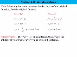
Antiderivatives • In each case, the problem is to find a function F whose derivative is a known function f. • If such a function F exists, it is called an antiderivativeof f. Definition • A function F is called an antiderivative of f on an interval I if F’(x) = f (x) for all x in I.
Antiderivatives • For instance, let f (x) = x2. • It is not difficult to discover an antiderivative of f if we keep the Power Rule in mind. • In fact, if F(x) = ⅓ x3, then F’(x) = x2 = f (x).
Antiderivatives • However, the function G(x) = ⅓ x3 + 100 also satisfies G’(x) = x2. • Therefore, both F and G are antiderivatives of f.
Antiderivatives • Indeed, any function of the form H(x)=⅓ x3 + C, where C is a constant, is an antiderivative of f. • The question arises: Are there any others? • To answer the question, recall that, in Section 4.2, we used the Mean Value Theorem. • We proved that, if two functions have identical derivatives on an interval, then they must differ by a constant.
Antiderivatives • Thus, if F and G are any two antiderivatives of f, then F’(x) = f (x) = G’(x) • So, G(x) – F(x) = C, where C is a constant. • We can write this as G(x) = F(x) + C. • Hence, we have the following theorem.
Antiderivatives • If F is an antiderivative of f on an interval I, the most general antiderivative of f on I is F(x) + C where C is an arbitrary constant. Theorem 1
Antiderivatives • Going back to the function f (x) = x2, we see that the general antiderivative of f is ⅓ x3 + C.
Family of Functions • By assigning specific values to C, we obtain a family of functions. • Their graphs are vertical translates of one another. • This makes sense, as each curve must have the same slope at any given value of x.
Notation for Antiderivatives • The symbol is traditionally used to represent the most general an antiderivative of f on an open interval and is called the indefinite integral of f . • Thus, means F’(x) = f (x)
Notation for Antiderivatives • For example, we can write • Thus, we can regard an indefinite integral as representing an entire family of functions (one antiderivative for each value of the constant C).
Antiderivatives – Example 1 • Find the most general antiderivative of each function. • f(x) = sin x • f(x) = 1/x • f(x) = xn, n ≠ -1
Antiderivatives – Example 1 • Or, which is basically the same, evaluate the following indefinite integrals: • . • . • .
Antiderivatives – Example 1a • If F(x) = – cos x, then F’(x) = sin x. • So, an antiderivative of sin x is–cos x. • By Theorem 1, the most general antiderivative is: G(x) = –cos x +C. Therefore,
Antiderivatives – Example 1b • Recall from Section 3.6 that • So, on the interval (0, ∞), the general antiderivative of 1/x is ln x + C. That is, on (0, ∞)
Antiderivatives – Example 1b • We also learned that for all x ≠ 0. • Theorem 1 then tells us that the general antiderivative of f(x) = 1/x isln|x| + C on any interval that does not contain 0.
Antiderivatives – Example 1b • In particular, this is true on each of the intervals (– ∞, 0) and (0, ∞). • So, the general antiderivative of f is:
Antiderivatives – Example 1c • We can use the Power Rule to discover an antiderivative of xn. • In fact, if n ≠ -1, then
Antiderivatives – Example 1c • Therefore, the general antiderivative of f (x) = xn is: • This is valid for n ≥ 0 since then f (x) = xn is defined on an interval. • If n is negative (but n ≠ -1), it is valid on any interval that does not contain 0.
Indefinite Integrals - Remark • Recall from Theorem 1 in this section, that the most general antiderivative on a given interval is obtained by adding a constant to a particular antiderivative. • We adopt the convention that, when a formula for a general indefinite integral is given, it is valid only on an interval.
Indefinite Integrals - Remark • Thus, we write with the understanding that it is valid on the interval (0,∞) or on the interval (–∞,0).
Indefinite Integrals - Remark • This is true despite the fact that the general antiderivative of the function f(x) = 1/x2, x ≠ 0, is:
Antiderivative Formula • As in the previous example, every differentiation formula, when read from right to left, gives rise to an antidifferentiation formula.
Antiderivative Formula • Here, we list some particular antiderivatives.
Antiderivative Formula • Each formula is true because the derivative of the function in the right column appears in the left column.
Antiderivative Formula • In particular, the first formula says that the antiderivative of a constant times a function is the constant times the antiderivative of the function.
Antiderivative Formula • The second formula says that the antiderivative of a sum is the sum of the antiderivatives. • We use the notation F’ = f, G’ = g.
Indefinite Integrals • Any formula can be verified by differentiating the function on the right side and obtaining the integrand. For instance,
Antiderivatives – Example 2 • Find all functions g such that
Antiderivatives – Example 2 • First, we rewrite the given function: • Thus, we want to find an antiderivative of:
Antiderivatives – Example 2 • Using the formulas in the tables together with Theorem 1, we obtain:
Antiderivatives • In applications of calculus, it is very common to have a situation as in the example — where it is required to find a function, given knowledge about its derivatives.
Differential Equations • An equation that involves the derivatives of a function is called a differential equation. • These will be studied in some detail in Chapter 9. • For the present, we can solve some elementary differential equations.
Differential Equations • The general solution of a differential equation involves an arbitrary constant (or constants), as in Example 2. • However, there may be some extra conditions given that will determine the constants and, therefore, uniquely specify the solution.
Differential Equations – Ex. 3 • Find f if f’(x) = ex + 20(1 + x2)-1 and f (0) = – 2 • The general antiderivative of
Differential Equations – Ex. 3 • To determine C,we use the fact that f(0) = – 2 : f (0) = e0 + 20 tan-10 + C = – 2 • Thus, we have: C = – 2 – 1 = – 3 • So, the particular solution is: f (x) = ex + 20 tan-1x – 3
Differential Equations – Ex. 4 • Find f if f’’(x) = 12x2 + 6x – 4, f (0) = 4, and f (1) = 1.
Differential Equations – Ex. 4 • The general antiderivative of f’’(x) = 12x2 + 6x – 4 is:
Differential Equations – Ex. 4 • Using the antidifferentiation rules once more, we find that:
Differential Equations – Ex. 4 • To determine C and D,we use the given conditions that f (0) = 4 and f (1) = 1. • As f (0) = 0 + D = 4, we have: D = 4 • As f (1) = 1 + 1 – 2 + C + 4 = 1, we have: C = –3
Differential Equations – Ex. 4 • Therefore, the required function is: f (x) = x4 + x3 – 2x2 – 3x + 4
Graph • If we are given the graph of a function f, it seems reasonable that we should be able to sketch the graph of an antiderivative F. • Suppose we are given that F(0) = 1. • We have a place to start—the point (0, 1). • The direction in which we move our pencil is given at each stage by the derivative F’(x) = f (x).
Graph • In the next example, we use the principles of this chapter to show how to graph F even when we do not have a formula for f. • This would be the case, for instance, when f (x) is determined by experimental data.
Graph – Example 5 • The graph of a function f is given. • Make a rough sketch of an antiderivative F, given that F(0) = 2. • We are guided by the fact that the slope of y =F(x) is f (x).
Graph – Example 5 • We start at (0, 2) and draw F as an initially decreasing function since f(x) is negative when 0 < x < 1.
Graph – Example 5 • Notice f(1) = f(3) = 0. • So, F has horizontal tangents when x = 1 and x = 3. • For 1 < x < 3, f(x) is positive. • Thus, F is increasing.
Graph – Example 5 • We see F has a local minimum when x = 1and a local maximum when x = 3. • For x > 3, f(x) is negative. • Thus, F is decreasing on (3, ∞).