Download

1 / 23
240 likes | 464 Views
8- 1. Capital Structure and Valuation. Example. Capital Structure. Current. Proposed. Miller and Modigliani: Proposition I. Strategy A: Buy 100 shares of levered equity. Strategy B: Buy 200 shares of unlevered equity using $2,000 in borrowing (Homemade Leverage).

E N D
8-1 Capital Structure and Valuation
Capital Structure Current Proposed
Miller and Modigliani: Proposition I Strategy A: Buy 100 shares of levered equity Strategy B: Buy 200 shares of unlevered equity using $2,000 in borrowing (Homemade Leverage) Proposition I (no taxes): Value of the unlevered firm is equal to the value of the levered firm
Miller and Modigliani: Proposition II(no taxes) • Remember: rWACC = D/A × rD + E/A × rE • MM(I) implies rWACC is independent of leverage • Define r0 is cost of capital for all-equity firm • r0 = unlevered earnings / unlevered equity =15% • Result: r0=rWACC if there are no taxes • Result: MM(II) (no taxes): rE = r0 + D/E × (r0 – rD)
Cost of Capital and MM(2) Cost of Capital (%) rE r0 rWACC rD D/E
Taxes • Present value of the tax shield • Interest = rD × D • Tax reduction = Tc × rD × D • Under normal circumstances we can assume: • cash flow from tax reduction has same risk as debt • cash flows are perpetual • PV(Tax Shield) = (Tc × rD × D) / rD = Tc × D • MM(I): VL = VU + Tc × D • VU = (EBIT × (1 – Tc)) / r0
MM(2):rE = r0 + D/E × (1-Tc) (r0 – rD) Cost of Capital (%) rE A declining rWACC is a direct result from MM(I), i.e, the value of the firm rises in leverage r0 rWACC rD D/E
Example • Blue Inc. has no debt and is expected to generate $4 million in EBIT in perpetuity. Tc=30%. All after-tax earnings are paid as dividends.The firm is considering a restructuring, allowing $10 million in debt at an interest rate of 8%. The unlevered cost of equity, r0, is 18%. • What is the current value of Blue? • VU=EBIT × (1–Tc) / r0 = ($4 million × 0.7) / 0.18 = $15.56 million • What will the new value be after the restructuring? • VL = VU + Tc × D = $15.56 + 0.3 × $10 = $18.56 million • What will the new required return on equity be? • rE = 0.18 + (10/8.56) × 0.7 × (0.18 – 0.08) = 26.18% • Check with: Elevered = ((4 – 0.8) × 0.7) / 0.2618 = $8.56 million
How about using rWACC? • rWACC = (10/18.56) × 0.7 × 0.08 + (8.56/18.56) × 0.2618 = 15.08% • Hence, Blue has decreased its WACC from 18% to 15.08% • VL = (4 × 0.7) / 0.1508 = $18.56 million
Downside of DebtFinancial Distress and Agency Costs • Financial Distress costs decrease the size of the firm and hence decrease the distribution to shareholders and bondholders. • Costs • Direct costs of financial distress • Indirect costs of financial distress • Agency costs (of debt) • Asset substitution and risk shifting • Underinvestment • Milking the company
Static trade-off theory of debt Firm Value Maximum Firm Value Actual Firm Value Debt Optimal amount of Debt
More on Agency CostsBenefits of debt • Agency cost of Equity (motive) • Shirking is less likely when issuing debt • Perquisites are less likely with debt • Over-investment is less likely with debt • Agency cost of Free Cash Flow (opportunity) • Retained earnings versus dividends? • Growth and investment opportunities • Debt serves as a monitoring device, decreasing managerial discretion
The Pecking-Order Theory • Internal Financing • External Financing • Debt Financing • Equity Financing (last resort) • Asymmetric information and Signaling • Dynamic decision, rather than static
Valuation • Weighted Average Cost of Capital • All Cash Flows discounted by discount rate that takes into account leverage • Adjusted Present Value • Separate cash flows from project and cash flows from financing • Flow-to-Equity Approach • Cash flows to equity holders discounted by the cost of equity
Example • You are considering a project with the following characteristics: • Perpetual cash inflows starting in year 1 of $25,000 per year • Yearly operating expenses of 12% of revenues • Initial investment outlay of $125,000 • Tc=34% and r0=14%, rD=8% • Calculate the NPV for an all-equity firm • Calculate the NPV for a firm with a target capital structure of 65% debt and 35% equity • Use WACC method • Use APV method • Use FTE method
Answers • Unlevered firm valuation Cash Inflows $25,000 Operating Expenses $ 3,000 Operating Income $22,000 Tax $ 7,480 Unlevered Cash Flow (UCF) $14,520 To the shareholders NPV = –$125,000 + ($14,520 / 0.14) = –$21,286
Answer • WACC rWACC = (D/V) × (1–Tc) × rD + (E/V) × rE rWACC = (0.65) × (1– 0.34) × 0.08 + (0.35) × rE rE = r0 + (D/E) × (1 – Tc) × (r0 – rD) rE = 0.14+ (65/35) × (1 – 0.34) × (0.06) = 0.2135 = 21.35% rWACC = (0.65) × (1– 0.34) × 0.08 + (0.35) × 0.2135 = 10.906% NPV = –$125,000 + ($14,520 / 0.10906) = $8,138
Answer • APV NPV of Financing Side Effects APV = NPV + NPVF NPVF = Tc × D APV = –$21,286 + (0.34 × 0.65 × (APV + $125,000)) 0.779 × APV = $6,339 APV = $8,138 Verify the target capital structure: Firm borrows 0.65 × ($125,000 + $8,138) Firm borrows 0.65 × $133,137 = $86,539.52 Firm uses $125,000 – $86,539.52 = $38,460.48 in equity
Answer VL = VU + Tc × D VL = 125,000– 21,286 + 0.34 × 0.65 × VL VL = 133,138 D = 0.65 × 133,138 • FTE method Cash Inflows $25,000 Operating Expenses $ 3,000 Operating Income $22,000 Interest (8% of $86,539.52)$ 6,923 Income after interest $15,077 Tax $ 5,126 Levered Cash Flow (LCF) $ 9,951 To the shareholders From before, rE = 21.35% and PV = $9,951 / 0.2135 = $46,609 NPV = – $38,460 + $46,598 = $8,138
Evaluation • Valuation for all-equity firm is easy • Valuation for levered firm is complex • tax shields • bankruptcy, agency, and other costs • WACC, APV, and FTE method • constant risk over life of project (constant r0) • constant debt/value ratio over life of project (constant rE and rWACC) • FTE and WACC work well under this scenario • if debt/value ratio is changing use APV (based on the level of debt) • APV works well for LBO’s and cases with interest subsidies and flotation costs (see example in Appendix 17A).
Beta revisited • Remember the following: • LeveredEquity = L = Unlevered Assets × (1 + (D/E)) • Assumes Debt = 0and no corporate taxes • With corporate taxes (assume Debt = 0): • L = U × [1 + (1–Tc) × (D/E)] • Unlevered Firm < LeveredEquity Remember: RE > R0 > RD
What if Beta of debt 0? • L = U + [(1–Tc) × (U – D) × (D/E)] L = levered equity U = unlevered equity (100% equity firm) D = debt E = equity