Flame Temperature
Flame Temperature. 朱 信 Hsin Chu Professor Dept. of Environmental Engineering National Cheng Kung University. 1. Energy Balance on a System. A simple steady-state thermal energy balance can be constructed around a constant-pressure combustion system (such as a boiler).

Flame Temperature
E N D
Presentation Transcript
Flame Temperature 朱 信Hsin ChuProfessorDept. of Environmental EngineeringNational Cheng Kung University
1. Energy Balance on a System • A simple steady-state thermal energy balance can be constructed around a constant-pressure combustion system (such as a boiler). • Next slide (Fig. 4.1)The energy flows into and out of the system.
Before the energy balance is developed it is worth looking more closely at the terms involved:(a) HR, HP and CV (calorific value) are all related to the standard temperature of 25℃. The enthalpy of the entering air is considered to be sensible heat only (i.e., the fuel/air is considered to be a dry mixture).(b) The enthalpy of the flue gas must be consistent with the calorific value of the fuel which is used in the balance.
If the gross calorific value is used, then HR should contain a latent heat term equal to the mass of water produced per kilogram of fuel multiplied by the latent heat of evaporation of water at 25℃ (hfg). • If the net calorific value is used, then the flue gas enthalpy will consist of sensible heat terms only. • In this chapter we are concerned with predicting the temperature reached within the flame, hence the net calorific value/sensible heat terms system is the more appropriate.
The energy balance about the system can be written as: CV + HR = HP + Qc + Qu (1) • HR, the sensible heat in the air and fuel (ref. 25℃) is very small and often neglected. • The case loss from the outside of the plant, Qc, is also generally small compared to the other energy fluxes and is similarly often considered negligible.
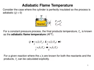
2. Adiabatic Flame Temperature • Table 4.1 shows flame temperatures for some common fuels. The higher the flame temperature, the greater should be the effectiveness of the heat exchanger section.
We can use the idea of the energy balance about the combustion system to derive a straightforward way of estimating the temperature of a flame. • It is assumed that combustion takes place under adiabatic conditions, i.e. no heat transfer is permitted across the boundary of the system.The implication of this is that Qc = 0 and Qu = 0 • Hence equation (1) simplifies down to CV + HR = HP (2)
It will be taken that CV is the net specific heat of the fuel, hence HP contains only sensible heat terms. • The terms on the left-hand side of equation (2) are simple to evaluate as CV will be known for the fuel used and HR, the enthalpy of the fuel and air (ref. 25℃), can easily be calculated fromWhere ti is the initial temperature.
The specific heats of the fuel, oxygen and nitrogen can be evaluated at the mean temperature (ti + 25)/2 and the enthalpy of the reactants is thus easily evaluated. • The right-hand side of equation (2), however, is not so easily evaluated as it is defined bywhere tf is the flame temperature. This relationship cannot be solved explicitly for tf as there will be a considerable difference between tf and the reference temperature 25℃, hence the value of tf is required to evaluate the specific heats of the combustion products.
3. Specific Heats of Gases • Simple ideal gas theory predicts that the specific heat of a gas is not a function of its temperature or pressure. • While the latter implication is effectively true in practice, the specific heat of a gas does increase with temperature above about 100℃. This effect arises because molecules have vibrational (internal) energy as well as kinetic energy due to the motion of the complete molecule.
This additional mode of “storing” energy will mean that the specific heat of a gas will increase as its temperature rises. • This cannot be modelled using the ideas of classical mechanics but the effect can be predicted using quantum theory.
Empirical equations which allow the calculation of specific heats as a function of temperature have been in use for some time. A polynomial expression is normally used, with either fractional or integer powers. • A straightforward integer power series is most convenient: CP = a[0] + a[1]t +a[2]t2 + a[3]t3 +…….. • Values for the coefficients for the polynomials for some gases are given in Table 4.2 (next slide and second slide).Where 9.9739 e-4 means 9.9739 × 10⁻⁴
In the case of the above values, the data was obtained in the temperatures range 25-2,000℃ and the polynomials should not be used outside these limits. • For hand calculations, tables of specific heats are a more useful formulation and Table 4.3 (next slide) gives values for the common combustion gases over a typical range of temperatures for combustion in boilers. • Straightforward linear interpolation should be used for intermediate temperatures.
4. Calculation Algorithm • A straightforward method for the calculation of adiabatic flame temperature is to execute the following steps:(1) evaluate the left-hand side of equation (2), i.e. (CV + HR); (2) guess a value for tf and use this to find the specific heats of the combustion products at the average between the flame and the reference temperature, i.e. [(tf + 25)/2]℃;
(3) solve equation (2) for tf;(4) compare the new value of tf with the original estimate and if there is a substantial difference use the new value to re-evaluate the specific heats, looping back to step (2) until satisfactory convergence is achieved.
With regard to step (2) above, taking the average temperature over the interval is only valid if the relationship between specific heat and temperature is linear. • We have seen that this is not in fact the case and an integrating calculation should be used. • However, the accuracy of calculating the adiabatic flame temperature by this simple procedure is constrained by a number of limitions, hence taking a simple arithmetical average is quite acceptable.
While this method is not a particularly efficient algorithm, it is stable and will generally converge to within 5℃ in four iterations. • Example 1:Find the adiabatic flame temperature for a stoichiometric methane/air flame if the initial temperature of the fuel and air is 10℃. Take the net calorific value of methane as 50.14 MJ/kg. • Solution:The first step is to evaluate, for 1 kg fuel, the mass of each of the reactants and products. These steps have been covered in previous chapters and the result can be summarized thus:
Reactants Products1 kg CH4 2.75 kg CO24 kg O2 2.25 kg H2O13.17 kg N2 13.17 kg N2The initial temperature of the reactants is 10℃ and the value of HR is the sensible heat in the reactants (ref. 25℃): HR = (10-25){1.CPCH4 + (4.CPO2) + (13.17.CPN2)} • The mean temperature of the reactants over the interval is 17.5℃. At this temperature the values of the specific heats are: CH4 2.23 kJ/kg/K O2 0.92 N2 1.04so HR = -293.9 kJ/kg methane
Giving HP = CV + HR =50,144 – 293.9 = 49,850 kJ/kgThis value of HP represents the sensible heat in the combustion products above the reference temperature of 25℃, i.e.49,850 = (tf - 25) {(13.17.CPN2) + (2.25.CPH2O) + (2.75.CPCO2)} • To solve this equation by trial and error requires an initial guess for the flame temperature.If we assume 1,575℃, the mean temperature of the products above 25℃ is (1,575 + 25)/2, i.e. 800℃.
The specific heats of nitrogen, water vapor and carbon dioxide at this temperature are N2 1.18 kJ/kg/K H2O 2.33 CO2 1.26so the energy equation is 49,850 = (tf-25){(13.17×1.18)+(2.25×2.33)+(2.75×1.26)}tf=2,081℃ • The new mean temperature of the products is (2,081+25)/2=1,053℃
The specific heats are now: N2 1.22 kJ/kg/K H2O 2.50 CO2 1.30solving the energy equation for the third time gives: tf = 1,998℃ • The mean temperature of the products now becomes (1,998+25)/2=1,012℃ giving N2 1.22 kJ/kg/K H2O 2.48 CO2 1.30A further evaluation of the energy equation gives tf = 2,001℃ #
5. Calculated Adiabatic Flame Temperatures • Values of the predicted adiabatic flame temperature for hydrocarbon fuels are affected by the following factors:(1) the calorific value (and chemical composition) of the fuel;(2) the air-to-fuel ratio at which combustion takes place; and(3) the initial temperature (preheat) of the air and fuel.
CALORIFIC VALUE • It would be expected that the higher the calorific value of the fuel the higher the final flame temperature produced.The picture is, however, not quite as simple as this since the chemical composition of the fuel also plays a part. • For example, natural gas has a carbon-to-hydrogen ratio of around 3.1 and a calorific value of 54 MJ/kg (gross). A typical coal, on the other hand, has a carbon-to-hydrogen ratio of around 18.0 and a calorific value of 33.3 MJ/kg.
Fuels with a higher proportion of hydrogen will generate more water vapor in their combustion products; a glance at Table 4.3 shows that water vapor has a higher specific heat than the other combustion products, which will lower the adiabatic flame temperature. • The adiabatic flame temperature for a number of common hydrocarbon fuels are given before in Table 4.1. In each case combustion is stoichiometric and the initial temperature of the air and fuel is 25℃.
It can be seen that there is quite a small variation in the calculated flame temperature, given the wide variation between the calorific values of these fuels. • The “conformity” is due to the effect of the hydrogen in the fuel discussed above.
AIR-TO-FUEL RATIO • Any excess air will increase the mass of flue gas relative to the mass of fuel, with a corresponding reduction in temperature. • With sub-stoichiometric air supply the flame temperature will also fall, as although the mass of flue gas is reduced, the effective calorific value of the fuel is also reduced by an amount equivalent to the calorific value of the carbon monoxide which is present in the flue gas.
The net calorific value of carbon monoxide is 10.11 MJ/kg. • Next slide (Fig. 4.2)It shows the temperature calculated for a natural gas flame as a function of the excess air ratio, and demonstrates the effects described above.
Very high flame temperature can be achieved by oxygen enrichment of the flame, as the mass of flue gas is considerably reduced. • Oxygen flames are used in a number of process applications, in particular welding, but the temperatures in oxygen-enriched flames are so high that dissociation effects (discussed later) are highly significant.
PREHEAT • Common sense (and equation (2)) suggest that preheating the air will increase the final temperature of the flame. • This is a useful feature because by increasing the temperature difference between the flue gas and the heat extracting fluid, greater heat transfer will be obtained for the same fuel input rate.
This will result in an increase in the thermal efficiency of the plant. • An example of the effect of preheat on the adiabatic temperature of a natural gas flame at 5% excess air is shown in Fig. 4.3 (next slide).
In practice, there are a number of reasons why the actual flame temperature will be lower than the value predicted by this procedure. • The most significant of these is that at the high temperature achieved in flames the combustion products will “dissociate” back into reactants or other higher reactive species: this process is accompanied by an absorption of energy, hence reducing the actual flame temperature.
The results of above calculations are then more correctly referred to as “undissociated adiabatic flame temperatures”, which acknowledges the simplifications inherent in them. • In order to understand the more complete picture it is necessary to gain some insight into the principles of chemical equilibrium, which are introduced in the next chapter.