Download
1 / 49
490 likes | 641 Views
V20 Topology of Protein Complexes on Graphs. (1) CombDock (2) Nuclear Pore Complex. Prediction Structures of Protein Complexes from Connectivities. CombDock: automated approach for predicting 3D structure of heterogenous multimolecular assemblies. Input : structures of N individual proteins

E N D
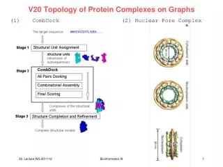
V20 Topology of Protein Complexes on Graphs (1) CombDock (2) Nuclear Pore Complex Bioinformatics III
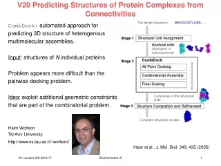
Prediction Structures of Protein Complexes from Connectivities CombDock: automated approach for predicting 3D structure of heterogenous multimolecular assemblies. Input: structures of N individual proteins Problem appears more difficult than the pairwise docking problem; it is NP-hard. Idea: exploit additional geometric constraints that are part of the combinatorial problem. Inbar et al., J. Mol. Biol. 349, 435 (2005) Bioinformatics III
Review: pairwise docking: Katchalski-Kazir algorithm Discretize proteins A and B on a grid. Every node is assigned a value Use FFT to compute correlation efficiently. Output: solutions with best surface complementarity. Gabb et al. J. Mol. Biol. (1997) Bioinformatics III
(1) All pairs docking module • Aim: predict putative pairwise interactions • Based on the N individual protein structures • perform pairwise docking for each of the • N (N - 1) / 2 pairs of proteins • Since the correct scoring of pairwise-docking • is difficult , the correct solution may be among • the first few hundred solutions. • keep K best solutions for each pair of proteins. • Here, K was varied from dozens to hundreds. Inbar et al., J. Mol. Biol. 349, 435 (2005) Bioinformatics III
(2) Combinatorial assembly module • Input: N subunits and N (N - 1) / 2 sets of K scored transformations. • These are the candidate interactions. • Reduction to a spanning tree • Spanning tree = a graph that connects all vertices and has no circles • Build weighted graph representing the input: • - each protein structure = vertex • each transformation (docking orientation) • = edge connecting the corresponding vertices • - edge weight = docking score of the transformation • Since the input contains K transformations for each pair of subunits, we get a complete graph with K parallel edges between each pair of vertices. Inbar et al., J. Mol. Biol. 349, 435 (2005) www.wikipedia.org Bioinformatics III
Spanning tree – algorithm of Kruskal Avoid constucting cycles Bioinformatics III
(2) Combinatorial assembly module For 2 subunits, each candidate binary docking complex is represented by an edge and the 2 vertices. For the full complex, a candidate complex is represented by a spanning tree. Each spanning tree of the input graph represents a particular 3D structure for the complex of all input structures. Problem of finding 3D structures of complexes is equivalent to finding spanning trees. The number of spanning trees in a complete graph with N nodes and no parallel edges is NN-2 (Cayley‘s formula). Here, the input graph has K parallel edges between each pair of vertices. the number of spanning trees is NN-2 KN-1 . Exhaustive searches are infeasible! Inbar et al., J. Mol. Biol. 349, 435 (2005) Bioinformatics III
(2) Combinatorial assembly module:algorithm • Algorithm uses 2 basic principles: • (1) hierarchical construction of the spanning tree • (2) greedy selection of subtrees • connect 2 subtrees of smaller size (that were previously generated) with an input edge to generate trees with i vertices • In this way, the common parts of different trees are generated only once. • When connecting subtrees, validate only the inter-subtree constraints. • check whether there are severe penetrations between pairs of subunits • that are represented by a different subtree. Inbar et al., J. Mol. Biol. 349, 435 (2005) Bioinformatics III
(2) Combinatorial assembly module:algorithm Stage 1: algorithm start with trees of size 1. Each tree contains a single vertex that represents a subunit. Stage i: the tree complexes that consist of exactly i vertices (subunits) are generated by connecting 2 trees generated at a lower stage with an input edge transformation. Tree complexes that fulfil the penetration constraint are kept for the next stages. Because it is impractical to search all valid spanning trees, the algorithm performs a greedy selection of subtrees. For each subset of vertices, the algorithm keeps only the D best-scoring valid trees that connect them. The tree score is the sum of its edge weights. Inbar et al., J. Mol. Biol. 349, 435 (2005) Bioinformatics III
Example The arp2/3 complex consists of 7 subunits (top). The figure shows only the complexes of the different stages that were relevant to the construction of the third-best scoring solution with RMSD 1.2 Å ) (bottom). The combinatorial assembly algorithm is hierarchical: at the first stage, each complex consists of a single subunit. At the i-th stage it constructs complexes that consist of i subunits by connecting complexes of smaller size using one of the input candidate transformations. Red edge: transformation of the current stage, Blue edges: transformations of previous stages. Inbar et al., J. Mol. Biol. 349, 435 (2005) Bioinformatics III
Final scoring A geometric score evaluates the shape complementarity between the subunits: - check distances between surface points on adjacent subunits. - close surface points increase score, - penetrating surface points decrease score. Physico-chemical component of the final score counts all surface points that belong to non-polar atoms = this gives an estimate of the hydrophobic effect. Inbar et al., J. Mol. Biol. 349, 435 (2005) Bioinformatics III
Clustering of solutions Clustering of solutions: (1) compute contact maps between subunits: array of N ( N – 1 ) bins. If two subunits are in contact within the complex, set the corresponding bit to 1, and to 0 otherwise. (2) superimpose complexes that have the same contact map and compute RMSD between C atoms. If this distance is less than a threshold, consider complexes as members of a cluster. For each cluster, keep only the complex with the highest score. Inbar et al., J. Mol. Biol. 349, 435 (2005) Bioinformatics III
Performance for known complexes Inbar et al., J. Mol. Biol. 349, 435 (2005) Bioinformatics III
Examples of large complexes CombDock solution solution superposed on the crystal structure (gray thiner lines) • the bestranked complex of the 10 subunits of RNA polymerase II, RMSD 1.4 Å. • (b) the third-best scoring assembly of the 7 subunits of the arp2/3 complex, RMSD 1.2 Å ; Inbar et al., J. Mol. Biol. 349, 435 (2005) Bioinformatics III
Discussion of CombDock For the 5 different targets, CombDock predicted at least 1 near-native solution and ranked it in the top 10 for both bound and unbound cases. Problem in evaluating performance: full sets of „unbound“ structures are often not available for complexes with a higher number of subunits. It is unlikely that this version of the algorithm (using rigid protein conformations) will be able to correctly assemble complexes de novo from unbound structures if the input subunits involve significant conformational changes. future version should include hinge-bending movements of protein subunits. Inbar et al., J. Mol. Biol. 349, 435 (2005) Bioinformatics III
Alber et al., Nature 450, 683 (2007) Bioinformatics III
The nuclear pore complex (NPC) NPCs are large assemblies of ca. 30 different proteins, the nucleoporins (ca. 120 megadaltons in metazoa). Each NPC contains at least 456 individual protein molecules. Surface rendered representation of a segment of nuclear envelope (NPCs in blue, membranes in yellow). The dimensions of the rendered volume are 1680 nm 984 nm 558 nm. The number of NPCs was ca. 45/m2. Nucleocytoplasmic transport of macromolecular cargoes between the nucleus and the cytoplasm depends on their recognition by transport factors (exportins and importins). These interact with the NPC to carry cargoes across the nuclear envelope. NPCs show a broad degree of compositional and structural conservation among all eukaryotes studied. Beck et al. Science 306, 1387 (2004) Bioinformatics III
Structure of the Dictyostelium NPC (A) Cytoplasmic face of the NPC in stereo view. The cytoplasmic filaments are arranged around the central channel. (B) Nuclear face of the NPC in stereo view. The distal ring of the basket is connected to the nuclear ring by the nuclear filaments. (C) Cutaway view of the NPC. Beck et al. Science 306, 1387 (2004) Bioinformatics III
Nuclear Pore Complex CryoEM shows the NPC as a doughnut-shaped structure with an eight-fold rotational axis perpendicular to the NE plane. This symmetry indicates that the NPC is composed of 8 identical building blocks, termed spokes arranged radially around a central channel that serves as the conduit for macromolecular transport. Each NPC spans the nuclear envelope through a pore formed by the fusion of the inner and outer nuclear envelope membranes. Numerous filamentous structures project from the NPC into the cytoplasm and nucleoplasm. The NPC consists of 30 different proteins. Bioinformatics III
4-level hierarchical representation of the NPC ImmunoEM experiments localized each nup to the nucleoplasmic, cytoplasmic, or both sides of the equatorial plane formally represent the NPC composition and protein stoichiometry with a 4-level hierarchy, consisting of - the whole NPC (assembly, A), - the 16 half spokes (unit, U), - the nup (protein, P), - and bead (particle, B) levels. Each of the 8 half-spoke units U at the cytosolic side is composed of 27 different types of nups, of which 2 are present in 2 copies each, totaling 29 protein instances. Similarly, each of the 8 half-spoke units U at the nucleoplasmic side contains 28 protein instances of 25 different types. 8 x (29 + 28) = 456 proteins in total Bioinformatics III
Overview of integrative structure determination Our approach to structure determination can be seen as an iterative series of 4 steps: - data generation by experiment, - translation of the data into spatial restraints, - calculation of an ensemble of structures by satisfaction of these restraints, and - an analysis of the ensemble to produce the final structure. The structure calculation part of this process is expressed as an optimization problem, a solution of which requires three main components: (1) a representation of the assembly in terms of its constituent parts; (2) a scoring function, consisting of individual spatial restraints that encode all the data; and (3) an optimization of the scoring function, which aims to yield structures that satisfy the restraints. Bioinformatics III
Dimensions and symmetry Top : the dimensions of the nuclear envelope, as taken from cryo-EM images. Bottom-left: the coordinate system used has the origin at the centre of the nuclear envelope pore. The nuclear envelope is indicated in grey. Bottom-right: the eight-fold (C-8) and two-fold (C-2) symmetry axes of the NPC, as revealed primarily by cryo-EM. Bioinformatics III
Stochiometry of each component in the NPC Aim: E.g. identification of Nup82 copy number. Aliquots of nuclear envelope preparations from PrA tagged strains equivalent to 3.6, 6, 10 and 15 μg were processed for immunoblot analysis. Result: Nup82 falls into the same range as the values of the 2 copy per spoke Nups. Strains with known copy numbers – Nup42, Nup1 (1 copy per spoke), Nup57, Nup84, Nup85 (2 copies per spoke) and Nsp1 (4 copies per spoke) were used as a control. Bioinformatics III
Shape and size of each component No atomic structures for most nucleoporins, estimate their shapes based on their sedimentation coefficients determined by ultracentrifugation of the purified proteins. Good: the sedimentation behaviour of most FG nucleoporins agrees with their predicted filamentous, native disordered structure. Good: Pom152, an integral membrane component, with multiple domains modelled as b-cadherin-like folds, appeared to be a highly elongated structure, consistent. Most of the other nucleoporins appear to have a relatively compact 3D structure in agreement with their predicted fold assignments. Bioinformatics III
Protein representation Every protein P is represented as a set of beads B, each with associated attributes (e.g., radius, mass). The number of beads and their attributes determine the resolution (granularity) of the protein representation. The most detailed data about the shape of most nups come from hydrodynamic experiments approximate the coarse shape and volume of each protein with a linear chain of equally-sized beads that best reproduce the observed sedimentation coefficients and are also consistent with our 3D fold assignments. Protein conformations in the NPC may differ from their conformations in solution. Therefore each protein is represented as a flexible chain, to allow for maximally extended to maximally compact conformations. The bead chain describes a protein at the highest resolution in our representation (the “root” representation κ = 1). Bioinformatics III
Protein shape from hydrodynamic experiments Shown are the stoichiometry of a protein in the cytoplasmic (cyt.) and nucleoplasmic (nucl.) half-spoke, as measured by quantitative immunoblotting. Smax values were calculated based on the molecular mass (kDa) of each protein; Smax/Sobs < 1.4 indicates a globular protein; 1.6–1.9, moderately elongated; > 2, highly elongated. Bioinformatics III
Localization of each component in the NPC The coarse localization of most nucleoporins within the NPC was obtained by immuno-EM, relying on a gold-labelled antibody that specifically interacted with the localized protein through its carboxy-terminal PrA tag. Immuno-EM montages for Pom152–PrA nuclei and Ndc1–PrA nuclear envelopes. Right: the position of every gold particle in each montage was measured from both the central Z-axis of the NPC (R) and from the equatorial plane of the nuclear envelope (Z). Bioinformatics III
Localization of each component in the NPC Estimated position of the C terminus of each protein in the NPC relative to the central Z-axis of the NPC (R) and the equatorial plane (Z) superimposed on the protein density map of a cross-section of the yeast NPC obtained by cryo-EM. Bioinformatics III
How do the NPC components fit together? The coarse shape, approximate position and stoichiometry of each nucleoporin are not enough to build an accurate picture of the NPC. Like the pieces in a jigsaw puzzle, we also need information about physical interactions between nucleoporins. Obtain information about interactions from overlay assays and affinity purification experiments, as well as from the composition of the Pom rings (consisting of Pom34 and Pom152). Overlay assay: identifies a pair of proteins that interact with each other. Affinity purification: identifies one or more proteins that interact directly or indirectly with the bait protein. An affinity purification produces a distinctive set of co-isolating proteins, which we term a composite. A composite may represent a single complex of physically interacting proteins or a mixture of such complexes overlapping at least at the tagged protein. Bioinformatics III
Protein interactions of the Nup84 complex above lanes: name of PrA-tagged protein and identification number for composite Below each lane: identity of co-purifying proteins; PrA-tagged proteins are blue, co-purifying nucleoporins black, NPC-associated proteins grey, and other proteins (e.g. contaminants) red. Affinity-purified PrA-tagged proteins and interacting proteins were resolved by SDS–PAGE and visualized with Coomassie blue. Molecular mass standards (kDa) are indicated to the left of the panel. The bands marked by filled circles at the left of the gel lanes were identified by mass spectrometry. Bioinformatics III
Localization of each component in the NPC A good example of the compositional overlap is the Nup84 complex. The smallest building blocks of this complex are heterodimers (composites 7, 14, 15). Under different isolation conditions, these dimers can be purified with an increasing number of additional proteins, such as trimers (25, 20), a tetramer (33), a pentamer (39), hexamers (44, 45, 51), and the full septameric Nup84 complex (53, 54, 57). This full complex interacts with Nup157 (63, 66) and Nup145N (60). Finally, the entire Nup84 complex coprecipitates together with the Nup170 complex and an Nsp1-containing complex (79). Bioinformatics III
Protein interactions of the Nup84 complex The mutual arrangement of the Nup84-complex-associated proteins as visualized by their localization volumes the final NPC structure. Bioinformatics III 33
Protein proximity by affinity purification + Composites determined by affinity purification. Vertical: affinity-purified nucleoporin–PrA Horizontal: corresponding nucleoporins in each composite. Right: composite identifiers Black box: indicates presence of a nucleoporin in a composite, Grey box: tagged nucleoporin. Dark grey box: a direct interaction determined by overlay assay. Bioinformatics III
Ambiguity in data interpretation and conditional restraints Shown is the ambiguity for a protein interaction between proteins of green and yellow types. The ambiguity results from the presence of multiple copies of the same protein in the same or neighbouring symmetry unit. In our NPC calculations, both neighbouring half-spokes on the cytoplasmic and nucleoplasmic sides are considered, for a total of four neighbouring half-spokes. Bioinformatics III
b, The conditional restraint is illustrated by an example of a composite of four protein types (yellow, blue, red, green), derived from an assembly containing a single copy of the yellow, blue, and red protein and two copies of the green protein; proteins are represented by a single bead (blue protein), a pair of beads (green and red proteins), and a string of three beads (yellow protein) (right panel). This composite implies that at least 3 of the following 6 possible types of interaction must occur: blue–red, blue–yellow, blue–green, red–green, red–yellow and yellow–green. In addition, (1) the 3 selected interactions must form a ‘spanning tree’ of the ‘composite graph’; (2) each type of interaction can involve either copy of the green protein; and (3) each protein can interact through any of its beads. These considerations can be encoded through a tree-like evaluation of the conditional restraint. At the top level, all optional bead–bead interactions between all protein copies are clustered by protein types. Each alternative bead interaction is restrained by a harmonic upper bound on the distance between the beads; these are ‘optional restraints’, because only a subset is selected for contribution to the final value of the conditional restraint. Next, a ‘rank-and-select’ operator (ORS) selects only the least violated optional restraint from each interaction type, resulting in six restraints (thick red line) at the middle level of the tree. Finally, the minimal spanning tree operator (OMST) finds the combination of 3 restraints that are most consistent with the composite data (thick red line); here the edge weights in the minimal spanning tree correspond to the restraint values given the current assembly structure. The column on the right shows a structural interpretation of the composite with proteins represented by their coloured beads and alternative interactions indicated by edges between them. The composite graph (left) is a fully connected graph that consists of nodes for all identified protein types and edges for all pairwise interactions between protein types; in the context of the conditional restraint, the edge weights correspond to the restraint values. 5 of the 16 possible spanning trees are also shown. This restraint evaluation process is executed at each optimization step based on the current configuration, thus resulting in possibly different subsets of selected optional restraints at each step. Bioinformatics III
Calculation of the NPC bead structure by satisfaction of spatial restraints Representative configurations at various stages of the optimization process from left (very large scores) to right (with a score of 0); a score of 0 indicates that all input restraints have been satisfied. The contact similarity quantifies how similar 2 configurations are in terms of the number and types of their protein contacts; a contact between two proteins occurs if the distance between their closest beads is less than 1.4 times the sum of the bead radii. Representation of the optimization process as it progresses from an initial random configuration to an optimal structure. As the score approaches zero, the contact similarity increases, showing that there is only a single cluster of closely related configurations that satisfy the input data. Bioinformatics III
Simulation protocol Bioinformatics III
Figure legend: Optimization in two stages First, a coarse sampling protocol (left column) generates 200,000 coarse configurations, starting each time from a different random configuration. This protocol relies on a variable target function method that consists of gradually increasing the number of restraints that are included in the scoring function, finally culminating in the full scoring function F. At each stage of the variable target function method, a combination of the conjugate gradient (CG) minimization and a molecular dynamics (MD) simulation with simulated annealing is applied. In total, a single optimization of an initial random configuration consists of an iteration of approximately 10.000 small shifts of protein particles (guided by either CG or MD). Second, a refinement protocol (right column) further refines the best 10% configurations from the sampling stage. Bioinformatics III
Final bead models a, Top: 2 representative bead models of the NPC (excluding the FG-repeat regions) from the ensemble of 1,000 superposed structures satisfying all restraints. The 8 positions of 3 sample proteins (Nup192, Nup57 and Nup85) on the cytoplasmic side are shown, with a detailed view of the bead representation of 1 copy of Nup85 at the bottom. Bioinformatics III
localization volumes Ensemble interpretation in terms of protein positions, contacts and configuration. a, Localization volumes of all 456 proteins in the NPC (excluding the FG-repeat regions) in 4 different views. Bioinformatics III
Contact frequencies for all pairs of proteins Contact frequency : fraction of structures in the ensemble that contains at least one protein contact between any protein instances of the 2 types. Bioinformatics III
Contact frequencies between proteins in composite 40 Proteins are nodes connected by edges with the observed contact frequency as the edge weight (indicated by its thickness). Edges that are part of the maximal spanning tree are shown by thick blue lines. The maximal spanning tree is the spanning tree that maximizes the sum of the edge weights. Dotted red lines: edges with a statistically significant reduction in contact frequency from their initial values implied by the composite data alone (P-value <10-3). Bioinformatics III
Protein adjacencies Protein adjacencies for the whole NPC, with 30 proteins as nodes and edges connecting proteins that are determined to be adjacent to each other. The edge weight is the observed contact frequency. Bioinformatics III
Bead model, ensemble, localization probability The structure is increasingly specified by the addition of different types of synergistic experimental information. As an example, each panel illustrates the localization of 16 copies of Nup192 in the ensemble of NPC structures, generated using the data sets indicated below. The localization probability is contoured at 65% of ist maximal value (red). The smaller the volume, the better localized are the proteins. Bioinformatics III
Protein contacts Contact frequencies reflect the likelihood that a protein interaction is formed given the data considered and are calculated from the ensemble of optimized structures. Prediction of protein interactions from contact frequencies improves as more data are used. This figure shows as an example the contact frequencies between proteins found in composite 34. Contact frequencies are shown as edge weights and indicated by the thickness of the lines connecting the proteins. Left: only a single composite is used (together with stoichiometry and symmetry information), all interactions are equally likely. Middle: the highest likelihood of interaction between a particular protein pair from all composites is used, the uncertainty about the interactions is reduced. Right: all data are used, the contact frequencies are either very high (>0.65) or very low (<0.25), thus allowing a strong prediction of protein interactions. As before, numbers in red indicate final contact frequencies that significantly decreased (at a P-value <10-3) from their initial values. Bioinformatics III
Evaluation by experimental data not used sofar Finally, the structure was tested by comparing it to experimental data that were not included in the structure calculation. 1 omission of a randomly chosen subset of 10% of the protein interaction data still results in structures with contact frequencies essentially identical to those derived from the complete data set the structure is robust. 2 the shape of our NPC structure strongly resembles the published EM maps of the NPC, even though these data were not used here. 3 the diameter of the transport channel in our structure is ca. 38nm (excluding the FG-repeat regions), in good agreement with the experimentally reported maximal diameter of transported particles. 4 Nup133, which has been experimentally shown to interact with highly curved membranes via its ALPS-like motif, is adjacent to the nuclear envelope in our structure. 5 Our configuration for Nup84 complex is completely consistent with previous results. Bioinformatics III
Evaluation by experimental data not used sofar Frank Alber: „Together these assessments indicate that our data are sufficient to determine the configuration of the proteins comprising the NPC. Indeed, it is hard to conceive of any combination of errors that could have biased our structure towards a single solution that resembles known NPC features in so many ways.“ Bioinformatics III
Conclusions Integrative approach to solve the structure of an extremely large supracomplex using diverse biophysical and proteomic data. Advantages: 1 it benefits from the synergy among the input data. Data integration is in fact necessary for structure determination. None of the individual data sets contains sufficient spatial information on its own. 2 the integrative approach can potentially survey all the structures that are consistent with the data. Alternatively, if no structure is consistent with the data, then some experiments or their interpretations are incorrect. 3 this approach can make the process of structure determination more efficient, by indicating which measurements would be most informative. 4 the approach can, in principle, incorporate essentially any structural information about a given assembly. Thus, it is straightforward to adapt it for calculating higher resolution structures by including additional spatial restraints from higher resolution data sets, such as atomic structures of proteins, chemical crosslinking, footprinting, small angle X-ray scattering (SAXS) and cryo-EM. Bioinformatics III