Download
1 / 48
480 likes | 622 Views
Protein complexes play a crucial role in cellular processes, enhancing enzymatic efficiency through close interactions. Various enzymes in biochemical pathways can assemble into larger complexes, improving substrate transfer and localizing reaction sites. Membrane transporters may oligomerize, allowing regulated structure formation. RNA polymerase II is essential for gene expression, synthesizing mRNA in eukaryotes. Additionally, ribosomes, the sites of protein synthesis, and the nuclear pore complex, which regulates macromolecule transport, are key components of cellular architecture. This overview highlights these fundamental protein complexes and their functions.

E N D
V18: Protein complexes – Density fitting (1) We normally assume that various enzymes of a biochemical pathway „swim“ in the cytosol and randomly meet the substrate molecules one after another. Yet, sometimes multiple enzymes of a pathway associate into large complexes and „hand over“ the substrates from one active site to the next one. Advantage: avoids free diffusion, increases local substrate density. (2) Membrane transporters and receptors often form oligomers in the membrane. Advantage: (i) large structures are built from small building blocks (simplicity) (ii) Oligomer formation can be regulated separately from transcription. (3) Also: complicated structural components of the cell (e.g. cytoskeleton) are built from many small components (e.g. actin) Bioinformatics III
RNA Polymerase II RNA polymerase II is the central enzyme of gene expression and synthesizes all messenger RNA in eukaryotes. Cramer et al., Science 288, 640 (2000) Bioinformatics III
RNA processing: splicesome Structure of a cellular editor that "cuts and pastes" the first draft of RNA straight after it is formed from its DNA template. It has two distinct, unequal halves surrounding a tunnel. Larger part: appears to contain proteins and the short segments of RNA, smaller half: is made up of proteins alone. On one side, the tunnel opens up into a cavity, which is believed to function as a holding space for the fragile RNA waiting to be processed in the tunnel. Profs. Ruth and Joseph Sperling http://www.weizmann.ac.il/ Bioinformatics III
Protein synthesis: ribosome The ribosome is a complex subcellular particle composed of protein and RNA. It is the site of protein synthesis, http://www.millerandlevine.com/chapter/12/cryo-em.html Model of a ribosome with a newly manufactured protein (multicolored beads) exiting on the right. Components of ribosome assemble spontaneously in vitro: No helper proteins (assembly chaperones) needed Bioinformatics III
Nuclear Pore Complex A three-dimensional image of the nuclear pore complex (NPC), revealed by electron microscopy. A-B The NPC in yeast. Figure A shows the NPC seen from the cytoplasm while figure B displays a side view. C-D The NPC in vertebrate (Xenopus). http://www.nobel.se/medicine/educational/dna/a/transport/ncp_em1.html Three-Dimensional Architecture of the Isolated Yeast Nuclear Pore Complex: Functional and Evolutionary Implications, Qing Yang, Michael P. Rout and Christopher W. Akey. Molecular Cell, 1:223-234, 1998 NPC is a 50-100 MDa protein assembly that regulates and controls trafficking of macromolecules through the nuclear envelope. Molecular structure: lecture V22 Bioinformatics III
Arp2/3 complex The seven-subunit Arp2/3 complex choreographs the formation of branched actin networks at the leading edge of migrating cells. (A) Model of actin filament branches mediated by Acanthamoeba Arp2/3 complex. (D) Density representations of the models of actin-bound (green) and the free, WA-activated (as shown in Fig. 1D, gray) Arp2/3 complex. Volkmann et al., Science 293, 2456 (2001) Bioinformatics III
icosahedral pyruvate dehydrogenase complex: a multifunctional catalytic machine Model for active-site coupling in the E1E2 complex. 3 E1 tetramers (purple) are shown located above the corresponding trimer of E2 catalytic domains in the icosahedral core. Three full-length E2 molecules are shown, colored red, green and yellow. The lipoyl domain of each E2 molecule shuttles between the active sites of E1 and those of E2. The lipoyl domain of the red E2 is shown attached to an E1 active site. The yellow and green lipoyl domains of the other E2 molecules are shown in intermediate positions in the annular region between the core and the outer E1 layer. Selected E1 and E2 active sites are shown as white ovals, although the lipoyl domain can reach additional sites in the complex. Milne et al., EMBO J. 21, 5587 (2002) Bioinformatics III
Apoptosome Apoptosis is the dominant form of programmed cell death during embryonic development and normal tissue turnover. In addition, apoptosis is upregulated in diseases such as AIDS, and neurodegenerative disorders, while it is downregulated in certain cancers. In apoptosis, death signals are transduced by biochemical pathways to activate caspases, a group of proteases that utilize cysteine at their active sites to cleave specific proteins at aspartate residues. The proteolysis of these critical proteins then initiates cellular events that include chromatin degradation into nucleosomes and organelle destruction. These steps prepare apoptotic cells for phagocytosis and result in the efficient recycling of biochemical resources. In many cases, apoptotic signals are transmitted to mitochondria, which act as integrators of cell death because both effector and regulatory molecules converge at this organelle. Apoptosis mediated by mitochondria requires the release of cytochrome c into the cytosol through a process that may involve the formation of specific pores or rupture of the outer membrane. Cytochrome c binds to Apaf-1 and in the presence of dATP/ATP promotes assembly of the apoptosome. This large protein complex then binds and activates procaspase-9. Bioinformatics III
Determining molecular 3D structures Experimental techniques: Dimensions proteins: 1 – 5 nm atoms: 0.1 – 0.5 nm bond stability covalent ca. 300 kJ/mol H-bonds: ca. 5 – 20 kJ/mol X-ray crystallography - applicability NMR - resulting information electron microscopy - resolution FRET - distortions AFM pulling - effort/cost ... Prediction techniques: Homology modelling, correlation based fitting, ab-initio modelling Bioinformatics III
X-ray crystallography Beam of photons (no mass), need high energy, method needs relatively large samples Bioinformatics III
X-ray reconstruction Bioinformatics III
Nuclear magnetic resonance Bioinformatics III
Electron microscopy (electrons have mass) (longer wavelength) Bioinformatics III
Atomic force microscopy Bioinformatics III
AFM pulling Can also be applied to protein complexes mutant Bioinformatics III
Fluorescence energy transfer Observed when CFP and YFP are far away Observed when CFP and YFP are close Bioinformatics III
Structural techniques - overview Bioinformatics III
Fitting atomistic structures into EM maps Bioinformatics III
The procedure Bioinformatics III
Step 1: blurring the picture Bioinformatics III
Put it on a grid Bioinformatics III
Fourier Transformation Bioinformatics III
Shift of the Argument Bioinformatics III
Convolution Integration in real space is replaced by simple multiplication in Fourier space. But FTs need to be computed. What is more efficient? Bioinformatics III
Fourier on a Grid + And so forth Bioinformatics III
FFT by Danielson and Lanczos (1942) Danielson and Lanczos showed that a discrete Fourier transform of length N can be rewritten as the sum of two discrete Fourier transforms, each of length N/2. One of the two is formed from the even-numbered points of the original N, the other from the odd-numbered points. Fke : k-th component of the Fourier transform of length N/2 formed from the even components of the original fj’s Fko : k-th component of the Fourier transform of length N/2 formed from the odd components of the original fj ’s Bioinformatics III
FFT by Danielson and Lanczos (1942) The wonderful property of the Danielson-Lanczos-Lemma is that it can be used recursively. Having reduced the problem of computing Fk to that of computing Fke and Fko , we can do the same reduction of Fke to the problem of computing the transform of its N/4 even-numbered input data and N/4 odd-numbered data. We can continue applying the DL-Lemma until we have subdivided the data all the way down to transforms of length 1. What is the Fourier transform of length one? It is just the identity operation that copies its one input number into its one output slot. For every pattern of log2N e‘s and o‘s, there is a one-point transform that is just one of the input numbers fn Bioinformatics III
FFT by Danielson and Lanczos (1942) The next trick is to figure out which value of n corresponds to which pattern of e‘s and o‘s in Answer: reverse the pattern of e‘s and o‘s, then let e = 0 and o = 1, and you will have, in binary the value of n. This works because the successive subdividisions of the data into even and odd are tests of successive low-order (least significant) bits of n. Bioinformatics III
Discretization and Convolution Bioinformatics III
Step 3: Scoring the Overlap Bioinformatics III
Cross Correlation Bioinformatics III
Correlation and Fourier 3 Bioinformatics III
Include convolution Bioinformatics III
Katchalski-Kazir algorithm Bioinformatics III
Discretization for docking Bioinformatics III
Docking the hemoglobin dimer Bioinformatics III
The algorithm Katchalski-Kazir et al. 1992 Algorithm has become a workhorse for docking and density fitting. Bioinformatics III
Problem I: limited contrast Bioinformatics III
Laplace filter Bioinformatics III
Enhanced contrast better fit Bioinformatics III
The big picture Bioinformatics III
Problem 2: more efficient search Bioinformatics III
Masked displacements Bioinformatics III
Rotational search Known Fourier coefficients of spherical harmonics Ylm. Bioinformatics III
Accuracy rmsd with respect to known atomistic structure of target. Bioinformatics III
Performance Bioinformatics III
Some examples Bioinformatics III
Summary • Today: • Docking into EM maps • - Discretization • - Correlation and blurring via FFT => Katchalski-Katzir algorithm • - Laplace filter => enhances contrast • - ADP_EM: FFT for rotations, scan displacements => better performance • Next lecture V19: • using connectivity information for complex assembly Bioinformatics III