Download
1 / 26
260 likes | 421 Views
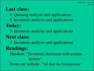
CDAE 266 - Class 24 Nov. 16 Last class: 4. Queuing analysis and applications 5. Inventory analysis and applications Today: 5. Inventory analysis and applications Next class: 5. Inventory analysis and applications Readings:

E N D
CDAE 266 - Class 24 Nov. 16 Last class: 4. Queuing analysis and applications 5. Inventory analysis and applications Today: 5. Inventory analysis and applications Next class: 5. Inventory analysis and applications Readings: Handout: “Inventory decisions with certain factors” From our website: “All Hail the Entrepreneur”
CDAE 266 - Class 24 Nov. 16 Important dates: Project 3 due today Problem set 5, due Tues., Dec. 5 Problems 6-1, 6-2, 6-3, 6-4, and 6-13 from the reading package Final exam: 8:00-11:00am, Thursday, Dec. 14
5. Inventory analysis and applications 5.1. Basic concepts 5.2. Inventory cost components 5.3. Economic order quantity (EOQ) model 5.4. Inventory policy with backordering 5.5. Inventory policy and service level 5.6. Production and inventory model
5.1. Basic concepts -- Inventories: parts, materials or finished goods a business keeps on hand, waiting for use or sell. -- Inventory policy (decision problems): Q = Inventory order quantity? R = Inventory reorder point (R = level of inventory when you make the order)? -- Optimal inventory policy: Determine the order quantity (Q) and reorder point (R) that minimize the inventory cost. -- SKU: Stock-keeping units
5.1. Basic concepts -- Lead time (L): the time between placing an order and receiving delivery -- Inventories models: (1) Economic order quantity (EOQ) model (2) Backordering model (3) Production and inventory model
5.2. Inventory cost components: -- Inventory ordering and item costs -- Ordering costs (telephone, checking the order, labor, transportation, etc.) -- Item cost (price x quantity) -- Inventory holding costs (interest, insurance, storage, etc.) -- Inventory shortage costs (customer goodwill and satisfaction costs)
5.3. The economic order quantity (EOQ) model 5.3.1. Assumptions: -- One item with constant demand (A) -- Lead time = 0 -- No backordering -- All the cost parameters are known
5.3. The economic order quantity (EOQ) model 5.3.2. A graphical presentation 5.3.3. Mathematical model -- Variable definitions: k = fixed cost per order A = annual demand (units per yr.) c = price h = annual holding cost per $ value T = time between two orders
A graphical presentation of the EOQ model: The constant environment described by the EOQ assumptions leads to the following observation THE OPTIMAL EOQ POLICY ORDERS THE SAME AMOUNT EACH TIME. Q Q Q This observation results in the inventory profile below:
5.3. The economic order quantity (EOQ) model 5.3.3. Mathematical model -- Assumptions: Constant demand No backordering
5.3. The economic order quantity (EOQ) model 5.3.3. Mathematical model -- Objective: choose order quantity (Q) to minimize the total annual inventory cost What is the reorder point (R)?
5.3. The economic order quantity (EOQ) model 5.3.3. Mathematical model -- Total annual inventory cost = annual ordering costs + annual holding cost + annual item costs (a) Annual order costs Annual demand = A Quantity of each order = Q Number of orders per yr. = A/Q Fixed cost per order = k Annual ordering costs = k (A/Q)
5.3. The economic order quantity (EOQ) model 5.3.3. Mathematical model -- Total annual inventory cost = annual ordering costs + annual holding cost + annual item costs (b) Annual holding costs Average inventory = Q/2 Annual holding cost per unit = hc Annual holding cost = (Q/2)*hc
Holding Costs (Carrying costs) Cost of capital Storage space cost Costs of utilities Labor Insurance Security Theft and breakage Annual unit holding cost h = Annual holding cost rate (cost per dollar value) c = Unit value (price) h * c
5.3. The economic order quantity (EOQ) model 5.3.3. Mathematical model -- Total annual inventory cost = annual ordering costs + annual holding cost + annual item costs (c) Annual item cost Average demand = A Cost per unit (price) = c Annual item cost = Ac
5.3. The economic order quantity (EOQ) model 5.3.3. Mathematical model -- Total annual inventory cost = annual order costs + annual holding cost + annual item costs -- Total annual relevant (variable) cost: -- Examples
5.3. The economic order quantity (EOQ) model 5.3.3. Mathematical model -- Derive the optimal solution: (1) A graphical analysis: the sum of the two costs is at the minimum level when the annual holding cost is equal to the annual ordering cost: => => =>
5.3. The economic order quantity (EOQ) model 5.3.3. Mathematical model -- Derive the optimal solution: (2) A mathematical analysis: At the minimum point of the curve, the slope (derivative) is equal to zero: => =>
5.3. The economic order quantity (EOQ) model 5.3.4. Reorder point if lead time > 0 If L > 0, R= L x A Note that L and A must have consistent units 5.3.5. Examples (1) Liquor store (pp. 209-211) Additional question: If the sale price is $3 per case, what will be the total “gross” profit per year?
5.3. The economic order quantity (EOQ) model 5.3.4. Examples (1) Liquor store (pp. 209-211) Available information: A = 5200 cases/yr k = $10/order c = $2 per case h = $0.20 per $ per yr. (a) Current policy: Q = 100 cases/order R = (5200/365) * 1 = 15 cases T = Q/A = 100/5200 (year) = 7 days TC = $540 per year (see page 210) (b) Optimal policy: Q* = 510 cases/order R = (5200/365) * 1 = 15 cases T = Q*/A = 510/5200 (year) =36 days TC = $204 per year If the retail price is $3 per case, Gross profit = 5200*3 – 5200*2 – 204 = $4996
Class exercise • 1. Draw a graph to show the following inventory policy for • a business with no backordering: the annual demand is • 3650 units and the business opens 365 days a year, the • order quantity is 305 units and the lead time is 4 days. • If some customers of the above business are willing to • take backorders and the maximum backorders are 50 units, draw another graph to show the inventory policy (there is no change in order quantity and lead time) • 3. Take-home exercise: Example on pp. 215-216 with the annual demand (A) increased to 1200 units and the lead time to be 3 days.
5.3. The economic order quantity (EOQ) model 5.3.5. Lead time (L), reorder point (R) and safety stock (SS) and their impacts (1) Inventory policy: Q: order quantity R: reorder point (Note that R is related to T but they are two different variables) (2) In the basic EOQ model: Q* = L = 0 ==> R* = L x A = 0 (3) If L > 0, R= L x A (the units of L & A must be consistent)
5.3. The economic order quantity (EOQ) model 5.3.5. Lead time (L), reorder point (R) and safety stock (SS) and their impacts (4) If the lead time is zero (L=0) and the co. wants to keep a safety stock (SS), R = L x A + SS = SS (5) If the lead time is greater than zero (L>0) and the co. wants to keep a safety stock, R = L x A + SS (6) Impacts of L & SS on R*, Q* and TC: No impact on Q* L ==> no impact on TC SS ==> increase TC by (hc * SS)
5.4. Inventory policy with backordering 5.4.1. A graphical presentation (page 214) A = Annual demand (e.g., 7300 kg per year) Q = order quantity [e.g., 200 kg per order (delivery)] S = Maximum on-hand inventory (e.g, 150 kg) Q - S = Maximum backorders (e.g., 50 kg) T = A/Q = time for each inventory cycle (e.g., T = 200/7300 = 0.0274 yr = 10 days) T1 = S/A = the time with on-hand inventory (e.g., T1 = 150/7300 = 0.0206 yr = 7.5 days) T2 = (Q-S)/A = T - T1 (e.g., T2= 50/7300 = 0.00685 yr = 2.5 days) T1/T = Proportion of time with on-hand inventory T2/T = Proportion of time without on-hand inventory Lead time and reorder point (e.g., L = one day)
5.4. Inventory policy with backordering 5.4.2. Total relevant (variable) inventory cost TC = annual ordering cost + annual holding cost + annual shortage (goodwill cost) = …… (see page 214) p = per unit goodwill (shortage) cost per year (e.g., p=$2 per unit per year) 5.4.3. Optimal inventory policy (page 215) Q* = S* = R =
5.4. Inventory policy with backordering 5.4.4. Example (pp. 215-216) A = 1000 cases of wine per year K = $100 per order (delivery) C = $20 per case h = $0.20 per dollar value per year p = $3.65 per unit of shortage per year L = 0 Q* = S* = R =