Proving Program Correctness: Axiomatic Approach to Partial and Total Correctness
This overview explores the axiomatic approach to proving program correctness, emphasizing the importance of partial and total correctness. We define correctness in terms of partial correctness (where a program meets its specification under certain conditions) and termination (complete correctness). The presentation includes a detailed discussion of computational modeling with predicates, axioms, and inference rules. Examples illustrate how to use predicates and axioms to prove program behaviors systematically, ensuring both the correctness of outputs and the termination of loops.

Proving Program Correctness: Axiomatic Approach to Partial and Total Correctness
E N D
Presentation Transcript
Proving Program Correctness The Axiomatic Approach
What is Correctness? • Correctness: • partial correctness + termination • Partial correctness: • Program implements its specification
Proving Partial Correctness • Goal: prove that program is partially correct • Approach: model computation with predicates • Predicates are boolean functions over program state • Simple example • {odd(x)} a = x {odd(a)} • Generally: {P} S {Q}, where • P precondition • Q postcondition • S Programming language statement
Proof System • Two elements of proof system • Axioms: capture the effect of prog. lang. stmts. • Inference rules: compose axioms to build up proofs of entire program behavior • Let’s start by discussing inference rules and then we’ll return to discussing axioms
Composition • Rule: • Consider two predicates • {odd(x+1)} x = x+1 {odd(x)} • {odd(x)} a = x {odd(a)} • What is the effect of executing both stmts? • {odd(x+1)} x = x+1 ; a = x {odd(a)}
Consequence 1 • Rule • Ex: • {odd(x)} a = x {odd(a)} and • Postcondition {a 4} • What can we say about this program?
Consequence 2 • Rule: • Ex: • Precondition {x=1} and • {odd(x)} a = x {odd(a)} • What can we say about this program?
Axioms • Axioms explain the effect of executing a single statement • Axioms will be derived “backwards.” • Start with postcondition and determine what conditions must be true on entry to stmt.
Assignment Axiom • Rule: • Replace all free occurences of x with y • e.g., {odd(x)} a = x {odd(a)}
Conditional Stmt 1 Axiom • Rule: {P} Bif {P Bif } {P Bif} S {Q}
Example: if even(x) then { x = x +1 } {odd(x) x > 3} else part (?? even(x) (odd(x) x>3) then part: {odd(x+1) x>2} x = x+1 {odd(x) x > 3} (?? even(x)) (odd(x+1) x>2) P ((odd(x+1) x>2) x >3) x > 3 works as well. Conditional Stmt 1
Conditional Stmt 2 Axiom • Rule {P} Bif {P Bif } {P Bif} S1 S2 {Q}
Example: if x < 0 then { x = -x; y = x else y = x } {y = |x|} Then part: {x = |x|} y = x {y = |x|} {-x = |x|} x = -x {x = |x|} ( ?? x <0) -x = |x| Else part: {x =|x|} y=x{y=|x|} ( ?? ¬(x < 0)) x = |x| P (-x = |x|) (x=|x|) Conditional Stmt 2 Axiom
While Loop Axiom • Rule • Infinite number of paths, so we need one predicate for that captures the effect of S • P is called an invariant {P} Bif S {P B}
Example IN {B 0} a = A b = B y = 0 while b > 0 do { y = y + a b = b - 1 } OUT {y = AB} INV y + ab = AB b 0 Bw b > 0 Show INV ¬ Bw OUT y + ab = AB b 0 ¬(b > 0) y + ab = AB b = 0 y = AB So {INV ¬ Bw} OUT Establish IN INV {ab = AB b 0} y=0 { INV} {aB = AB B 0} b = B {….} {AB = AB B 0} a = A {….} So {IN} a=A;b=B;y=0 {INV} While Loop Axiom
While Loop Axiom • Need to show {INV Bw} loop body {INV} {y+a(b-1) = AB b-1 0} b = b - 1 {INV} {y+a+a(b-1) = AB b-1 0} y = y+a {….} {y +ab = AB b-1 0} loop body {INV} • y + ab = AB b 0 b > 0 {y +ab = AB b-1 0}, • So • {IN} lines 1-3} {INV}, • {INV} while loop {INV ¬ Bw }, and • {INV ¬ Bw} OUT • Therefore • {IN} program {OUT}
Total correctness • After you have shown partial correctness • Need to prove that program terminates • Usually a progress argument. Last program • Loop terminates if b 0 • b starts positive and is decremented by 1 every iteration • So loop must eventually terminate