Coherence and decoherence in Josephson junction qubits
380 likes | 972 Views
Coherence and decoherence in Josephson junction qubits. Yasunobu Nakamura, Fumiki Yoshihara, Khalil Harrabi Antti Niskanen, JawShen Tsai. NEC Fundamental and Environmental Research Labs. RIKEN Frontier Research System CREST-JST. Decoherence of qubit, bias dependence

Coherence and decoherence in Josephson junction qubits
E N D
Presentation Transcript
Coherence and decoherence in Josephson junction qubits Yasunobu Nakamura, Fumiki Yoshihara, Khalil Harrabi Antti Niskanen, JawShen Tsai NEC Fundamental and Environmental Research Labs. RIKEN Frontier Research System CREST-JST • Decoherence of qubit, bias dependence • Tunable coupling scheme based on parametric coupling using quantum inductance
Charge qubit Flux qubit Phase qubit Energy typical qubit energy typical experimental temperature Josephson junction qubits small large Josephson energy = confinement potential charging energy = kinetic energy quantized states
2 mm Examples of Josephson junction qubits charge qubit/NEC flux qubit/Delft phase qubit/NIST/UCSB charge qubit (quantronium)/Saclay ~100 m
To hold voltage state after switching ~20 ns Ib pulse ~30 ns rise/fall time w/o -pulse time ~1 s switch w/ -pulse 0 SQUID readout of flux qubit qubit +underdamped SQUID SQUID 0 1 qubit I. Chiorescu, Y. Nakamura, C.J.P.M. Harmans, and J.E. Mooij, Science 299, 1869 (2003)
Coherent control of flux qubit Rabi oscillations resonant microwave pulse visibility~79.5%
Study of decoherence = Characterization of environment environment interaction qubit tunable tunable
magnetic-field noise? trapped vortices? paramagnetic/nuclear spins? charge fluctuations? • environment • circuit modes? phonons? • quasiparticle • tunneling? photons? charge/Josephson-energy fluctuations? Possible decoherence sources
f/f* f*=0.5 Flux qubit: Hamiltonian and energy levels J.E. Mooij et al. Science 285, 1036 (1999)
Sensitivity to noises relaxation transverse coupling dephasing longitudinal coupling
zero-point fluctuation of environment ex. Johnson noise in ohmic resistor R spontaneous emission absorption Energy relaxation relaxation and excitation for weak perturbation: Fermi’s golden rule • qubit energy E variable • relaxation S(+) and excitation S(-) • quantum spectrum analyzer
T1 measurement p ~ 4ns p readout pulse delay initialization to ground state is better than 90% relaxation dominant classical noise is not important at qubit frequency ~ 5GHz
T1 vs f p ~ 4ns delay readout pulse
1 vs E • Data from both sides of spectroscopy coincide • Positions of peaks are not reproduced in different samples • Peaks correspond to anticrossings in spectroscopy assuming flux noise (not assured)
1 vs E: Comparison of two samples sample5 sample3 Random high-frequency peaks. Broad low-frequency structure and high-frequency floor.
for Gaussian fluctuations sensitivity of qubit energy to the fluctuation of external parameter information of S() at low frequencies Dephasing free evolution of the qubit phase dephasing
spin echo p/2~2ns p/2 p ~ 4ns readout pulse t/2 t/2 Dephasing: T2Ramsey, T2echo measurement correspond to detuning Ramsey interference (free induction decay) p/2~2ns p/2 readout pulse t
E (GHz) Ib f Optimal point to minimize dephasing f • two bias parameters • External flux: f =ex/0 • SQUID bias current Ib Ib G. Burkard et at. PRB 71, 134504 (2005)
T1 and T2echo at f=f*, Ib=Ib* T1=54516ns Echo decay time is limited by relaxation Pure dephasing due to high frequency noise (>MHz) is negligible
Echo at ff*, Ib=Ib* assuming 1/f flux noise do not fit does not fit
Red lines: fit 2Ramsey, 2echo vs f For for 3.17 mm2 cf. 7±3x10⁻⁶ [F0] for 2500-160000 mm2 F.C.Wellstood et al. APL50, 772 (1987) ~1x10⁻⁴ [F0] for 5.6 mm2 G.Ithier et al. PRB 72, 134519 (2005)
Optimal point to minimize dephasing f • two bias parameters • External flux: f =ex/0 • SQUID bias current Ib Ib E (GHz) Ib f
T1, T2Ramsey, T2echo vs Ib can be obtained experimentally at Ib=Ib* at |Ib-Ib*|=large
Echo at f=f*, IbIb* at Ib=Ib* at |Ib-Ib*|=large -echo does not work -exponential decay white noise (cutoff>100MHz) exponential fit Gaussian fit
Optimal point f=f*, Ib=Ib* T1 limited echo decay Pure dephasing due to low freq. noise Sammary • T1, T2 measurement in flux qubit, T1,T2~1s • dependence on flux bias and SQUID-current bias condition • characterization of environment f=f*, IbIb* ‘white’ Ib noise dominant ff*, Ib=Ib* We do not understand yet -T1 vs flux bias -dephasing at optimal point -origin of 1/f noise 1/f flux noise dominant
At optimal point Dephasing is minimal Persistent current is zero Inductive coupling ~ xx; effective only for 12 Current readout should be done elsewhere Quantum inductance is finite Depend on flux bias tunable parametric coupling Depend on qubit state nondemolition inductance readout current inductance Optimal point and quantum inductance
Use nonlinear quantum inductance of high-frequency qubit3 as transformer loop Drive the nonlinear inductance at |1-2| and parametrically induce effective coupling between qubit1 and qubit2 Tunable coupling between flux qubits At the optimal point for qubit1 and qubit2 Effective coupling; can be zero at dc
Advantages Qubits are always biased at optimal point Coupling is proportional to MW amplitude; can be effectively switched off Induced coupling term also has protection against flux noise Tunable coupling between flux qubits |10 |01 Simulated time evolution vs. control MW pulse width Double-CNOT within tens of ns |10 |01 A.O. Niskanen et al., cond-mat/0512238
Three qubits and a readout SQUID 1 t |1-2| |00 |10 |10+|01 |00+|11 readout |00 Psw |11 t Simple demonstration of tunable coupling between flux qubits qubit3 qubit1 qubit2 Easy to distinguish |00 and |11 (not|01 and |10) A.O. Niskanen et al., cond-mat/0512238
Future Tunable coupling Nondemolition readout Single qubit control Long coherence time