Spin-Hamiltonian Analysis for a Pair of Spins Featuring Exchange and Spin-Spin Interactions
This document presents a comprehensive analysis of the Spin-Hamiltonian for a pair of spins, emphasizing the terms related to spin interactions, such as the Zeeman effect, exchange coupling, and anisotropic interactions. The mathematical framework outlines the effects of magnetic fields on the energy states of spin pairs, exploring different configurations and interactions. The significance of antiferromagnetic and ferromagnetic coupling, along with the pertinence of Goodenough-Kanamori rules in magnetic materials, is discussed, providing insights into magneto-structural correlations.

Spin-Hamiltonian Analysis for a Pair of Spins Featuring Exchange and Spin-Spin Interactions
E N D
Presentation Transcript
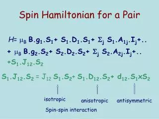
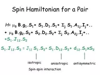
Spin Hamiltonian for a Pair H= BB.g1.S1+ S1.D1.S1+ j S1.A1j.Ij+.. + BB.g2.S2+ S2.D2.S2+ j S2.A2j.Ij+.. +S1.J12.S2 S1.J12.S2 = J12S1.S2+ S1.D12.S2+ d12.S1xS2 isotropic anisotropic antisymmetric Spin-spin interaction
S=0 Sa=1/2 E=Jex S=1 S= 5 S= 4 S= 3 S= 2 S= 1 S= 0 Energie degli stati S E(S)=(J/2)[S(S+1)-S1(S1+1)-S2(S2+1)]
Suscettività =
S=0 Sa=1/2 E=Jex S=1 Sa=1/2 e Sb=1/2 Sb=1/2 E(S=1)=1/2Jex(1*2-1/2*3/2-1/2*3/2)=-¼ Jex E(S=0)= 1/2Jex(-1/2*3/2-1/2*3/2)=3/4Jex E=Jex the energy of the four states are E(1,-1)=-gBH E(1,0)=0 E(1,1)=+gBH E(0,0)=Jex
Sa=1/2 e Sb=1/2 S=0 Sa=1/2 E=Jex Sb=1/2 E(S=1)=1/2Jex(1*2-1/2*3/2-1/2*3/2)=-¼ Jex E(S=0)= 1/2Jex(-1/2*3/2-1/2*3/2)=3/4Jex E=Jex 2Ng2B2 =------------------ kT[3+exp(Jex/kT)] eq. Bleaney - Bowers S=1
S=1 T= S=0 Magnetic field
S=1 T J/kB S=0 Magnetic field
Il modello di Anderson A-C-B →A+-C-B- Lo scambio cinetico favorisce il singoletto Lo scambio potenziale il tripletto
Regole di Goodenough-Kanamori • Se gli orbitali magnetici si sovrappongono l’accoppiamento è antiferromagnetico • Se gli orbitali magnetici sono ortogonali ed hanno ragionevoli zone di sovrapposizione lo scambio è ferromagnetico • Se un orbitale magnetico sovrappone con un orbitale vuoto l’accoppiamento è ferromagnetico
Interazione di scambio Orbitali magnetici (quelli che hanno l’elettrone spaiato) con sovrapposizione diversa da zero: accoppiamento antiferromagnetico
Interazione di scambio (2) Orbitali magnetici ortogonali: interazione ferromagnetica (regola di Hund)
Interazione di superscambio (3) La frazione di elettrone trasferita nell’orbitale z2 polarizza gli spin degli altri elettroni spaiati, tenendoli paralleli a sé: accoppiamento ferromagnetico
Alcuni Esempi: Dimeri di Rame(II) > 96° < 96° R.D.Willett, D.Gatteschi,O.Kahn, Magneto-Structural Correlations in Exchange Coupled Systems, NATO ASI C140,Reidel, 1985
Rame(II)-Vanadile(IV) Indipendente dall’angolo J> 100 cm-1
Un po’ di MO - Hay-Thibeault-Hoffman + J’ è l’integrale di scambio, k sono integrali coulombiani
Il modello di Kahn J=j-ks2 J integrale di scambio s integrale di sovrapposizione
Prussian Blue Type Compounds CnAp[B(CN)6]q.xH2O C monovalent cation A is N coordinated B is C coordinated The sign of the coupling can be easily understood considering the magnetic orbitals: if they are orthogonal the coupling is ferromagnetic, otherwise antiferromagnetic
Doppio Scambio L’elettrone passa dal Mn(III) al Mn(IV) mantenendo lo spin parallelo a quello degli altri elettroni: accoppiamento ferromagnetico
Doppio Scambio Mn3+ Mn4+
Un sistema a valenza mista di nichel Formalmente Ni(II)-Ni(I) Stato fondamentale S= 3/2. Nessuna evidenza di S= 1/2
Origin of the Spin-spin interaction • Through space (magnetic dipolar) • Through bonds (exchange)
Magnetic Dipolar J12dip= (B2/r3) [g1.g2- 3(g1.r)(g2.r)/r2]
Dipolar matrix in B2/r3 units gxxge 0 0 0 gyyge(1-3sin2) -3sin cos gyyge 0 -3sin cos gzzgegzzge(1-3cos2)
Decomposition of the interaction matrix J= (1/3)(Jxx+Jyy+Jzz) dxx=(Jyz-Jzy)/2 Dij=(Jij+Jji)/2
Dipolar interaction calculated r=2.5 Å r=3.5 Å r=4.5 Å J 18 7 3 D -3519 -1283 -603 E 28 11 5 dx -83 -30 -14 The values are given in 10-4 cm-1. gxx=gyy=2.2; gzz=2.0. The principal direction of D is parallel to the Mn-Cu direction
Origin of the Exchange Contributions J<g1g2Hexg1g2> D <n1g2Hexn1g2>2/2 D(g/g)2J d <n1g2Hexg1g2>/ d(g/g)J
SH Parameters for Pairs In the strong exchange limit, J>>D,d the total spin S=S1+S2 is a good quantum number: gS= c1g1+ c2g2 AS= c1A1+ c2A2 DS= d1D1+ d2D2+ d12D12 c1=(1+c)/2; c2= (1-c)/2; d1= (c++c-)/2; d2= (c+-c-)/2; d12= (1-c+)/2
Some numerical coefficients S1 S2 S c1 c2 d1 d2 d12 1/2 1/2 1 1/2 1/2 0 0 1/2 1 1 1 1/2 1/2 -1/2 -1/2 1 1 1 2 1/2 1/2 1/6 1/6 1/3 3/2 3/2 1 1/2 1/2 -6/5 -6/5 17/10 3/2 3/2 2 1/2 1/2 0 0 1/2 3/2 3/2 3 1/2 1/2 1/5 1/5 3/10
More coefficients S1 S2 S c1 c2 d1 d2 d12 2 2 1 1/2 1/2 -21/10 -21/10 13/5 2 2 2 1/2 1/2 -3/14 -3/14 5/7 2 2 3 1/2 1/2 1/10 1/10 2/5 2 2 4 1/2 1/2 3/14 3/14 2/7 5/2 5/2 1 1/2 1/2 -16/5 -16/5 37/10 5/2 5/2 2 1/2 1/2 -10/21 -10/21 41/42 5/2 5/2 3 1/2 1/2 -1/45 -1/45 47/90 5/2 5/2 4 1/2 1/2 1/7 1/7 5/14 5/2 5/2 5 1/2 1/2 2/9 2/9 5/18
And More S1 S2 S c1 c2 d1 d2 d12 1/2 1 1/2 -1/3 4/3 0 0 0 1/2 1 3/2 1/3 2/3 0 1/3 1/3 1/2 3/2 1 -1/4 5/4 0 3/2 -1/4 1/2 3/2 2 1/4 3/4 0 1/2 1/4 1/2 2 3/2 -1/5 6/5 0 7/5 -1/5 1/2 2 5/2 1/5 4/5 0 3/5 1/5 1/2 5/2 2 -1/6 7/6 0 8/6 -1/6 1/2 5/2 3 1/6 5/6 0 4/6 1/6
A test ground pair AF coupling J> 500 cm-1
Spin Hamiltonian Parameters gi= -1/6 g1i + 7/6 g2i