Download
1 / 25
250 likes | 444 Views
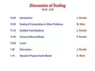
Discussion of Scaling 10:45 - 2:00. 10:45 Introduction J. Rundle 10:50 Scaling & Computation in Other Problems W. Klein 11:10 Scalable Fault Systems J. Rundle 11:50 Virtual California Model P. Rundle 12:00 Lunch 1:00 Discussion J. Rundle

E N D
Discussion of Scaling 10:45 - 2:00 10:45 Introduction J. Rundle 10:50 Scaling & Computation in Other Problems W. Klein 11:10 Scalable Fault Systems J. Rundle 11:50 Virtual California Model P. Rundle 12:00 Lunch 1:00 Discussion J. Rundle 1:15 Standard Physical Earth Model S. Ward
Hierarchy of Physical & Computational Spatial Scales A “system of systems” that scales with size in a predictable way, or “scalable fault system”
Scalable Earthquake Fault Systems Points for Discussion John Rundle University of Colorado, Boulder CO Presented at GEM-ACES Meeting, Maui HI, July 29-Augest 3, 2001 & SCEC2 Retreat, Lake Tahoe CA, July 20-22, 2001
Data-Model-Simulations Flow Diagram Earthquake Data: Fault Topology Plate Kinematics Stress Data Paleoseismology Current Seismicity Historic Events Locations Times Moment Tensors EQ Models: Physics of Friction & Local Instabilities Interactions & Stress Greens Functions Statistical & Stochastic Physics Nonlinear Dynamics EQ Simulations: Enabled by IT Algorithms Scalable Computing Grid Computing Web-based Object- Broker Systems Data Base Management Data Mining Visualization New Physics Falsifiable Tests New Data Predictions
A Strawman Definition of an Earthquake Fault System An earthquake fault system is a grouping of topologically complex faults or fault segments that have significant mutual interactions due to elastic or other stress transfer. The activity on the faults is strongly correlated and displays emergent space-time patterns that are properties of the system as a whole and not of the individual faults of which the system is composed. Scalable fault systems have physical properties and characteristic space-time patterns that depend on changes in spatial and temporal scales of resolution in predictable ways.
Scalable Physics and Computations 1. Earthquakes are a high dimensional complex system having many scales in space and time. Are all scales important? Or can we negelect some scales? 2. Do we need to use new approaches to the problem based on computational physics & information technology? - Earthquakes faults appear to be strongly correlated systems - Numerical simulations will allow us to understand & integrate the physics of earthquakes across all scales 3. Do scalable physics require scalable approaches to computations, data mining & visualization? - Correlation-Operator analysis - Hidden Markov Methods - Wavelets 4. Do we need to think about scalable computing? - Beowulf clusters (e.g., MPI, PVM) - Grid computing (e.g., www.gridcomputing.org, seti@home) - P2P architectures - Algorithms (e.g., Fast Multipoles)
Data base MyXoSServer MyXoSServer MyXoSServer MyXoSServer MyXoSServer ……. Sub scribe ….. Pu blish Peer to Peer P2P “Illusion” among collaborating clients High Performance Scalable Web-Based Computing P2P Modification of Client-Server Infrastructure Defines Framework for Multiscale Problem Solving Environment Publish / Subscribe: An asynchronous model of computation adaptable to web-based computing. MyXoS assumes an XML-type schema to describe objects, and the existence of an Object Request Broker middleware like CORBA
Serial & Parallel Codes Using MPI Parallel Code Using MPI Dimension Statements CALL MPI_INIT(ierrpr) CALL MPI_COMM_RANK(MPI_COMM_WORLD, myid, ierrpr) CALL MPI_COMM_SIZE(MPI_COMM_WORLD, nprocs, ierrpr) if (myid .eq. 0) then Enter some data end if call MPI_BCAST(variable_A,dimensions, MPI_DOUBLE_PRECISION, 0,MPI_COMM_WORLD,ierrpr) if (myid .eq. 0) then do statement over i call MPI_RECV(variable_B,dimensions, & MPI_DOUBLE_PRECISION, & MPI_ANY_SOURCE, MPI_ANY_TAG, & MPI_COMM_WORLD,status, ierrpr) end do else if (myid .ne. 0) then Do some computations Call a subroutine do statement over i call MPI_SEND(variable_B,dimensions, & MPI_DOUBLE_PRECISION,0, & i, MPI_COMM_WORLD,ierrpr) end do end if if (myid .eq. 0) then Print the answer end if call MPI_FINALIZE(ierrpr) End Code Serial Code Dimension Statements Enter some data Do some computations Call a subroutine Print the answer End Code MPI Send-Receive Block
A.D. 1857 1480 1812 1346 1680 1100 Historic Earthquakes on a Fault System Earthquakes on major faults occur quasi-periodically Major events on the San Andreas Fault From K. Sieh et al., JGR, 94, 603 (1989)
A Model for the Statistical Dynamics of an Earthquake Fault: The Burridge-Knopoff Slider Block Model R. Burridge and L. Knopoff, Bull. Seism. Soc. Am, 57, 341 (1967) Thenearest-neighbor BK modelwas the first slider block model. Sticking points on the fault are represented by blocks having uniform loader spring constantKL(= kp in figure at right). Each block is connected to its 2d nearest neighbors (d = spatial dimension) by springs having constantKC( =kc at right). Afriction lawprevents the blocks from sliding until sufficient force (stress) builds up. A simulated earthquake begins when the force on a block due to the plate motion reaches astress threshold F. The avalanche of failing blocks, triggered by stress transfer from sliding blocks, represents an earthquake.
K VLoad Rate of Change of Stress f( ,V) Stress, KL = 1.0, KC = 100.0, = 0.1, v = 0.48 Theoretical Friction Curves Can Be Obtained by Coarse- Graining Microscopic Dynamics in Space and TimeW. Klein et al., Phys. Rev Lett., 65, 1462, (1998) Macroscopic friction curves can be obtained by a space-time coarse-graining of the mean field slider block dynamics. Frictional sliding is a competition between the rate at which stress is supplied across the contact layer, K VLoad, and the rate at which stress is dissipated, f ( ) : d ()/ dt = K VLoad - f (,V) where: V = dS / dt , = - R . f ( ) has a Van der Waals loop, with two spinodal points (extrema...red arrows).
K VLoad f( ) Thermal Phase Transitions (Equilibrium) Frictional Sliding (Non-equilibrium) We Have An Apparent Paradox Here we see a non-equilibrium system that is demonstrating equilibrium properties...The appearance of spinodal loops, the spinodal scaling exponents, the form of the correlation function, and other properties. How does this physics arise?
F > 0 Stress R Time F = 0 Stress, R Recurrent Events:The Leaky Threshold Equations Recall: d / dt = K VLoad - f ( ) Expand f ( ) Leaky Threshold Equation (“Hopfield Equation”): d / dt = KVLoad - {+ i (t - tF,i)} Elasticity Equation: = K (VLoad t - S) Notes: 1. The - function parameterizes the sudden slip. 2. - R 3. ( t F) = F 4. { f / }T 5. S = slip Data from T Tullis, PNAS, 1996 (also see Karner & Marone, 2000)
F B K VM d C E f() dt D A Stress, Stress, K Model of Contact Layer Experiment Aside: Rate-State Friction can be Derived Consider the dynamical mean field equation: d ()/ dt = K V - f ( ) Figure: We expand around point C, having stress C and load velocity V = VM . Define: LM = { C - R } / K = VM / ( C ) Physically, LM is the shear displacement across the contact zone when = C - R Low stress stable branch AB Intermediate stress unstable branch BCD High stress stable branch DEF VM is Maxwell equal-area line We find from Rate-State experimental data: K .0025 MPa / m (Contact Layer Stiffness) VM1.26 mm/s (Maxwell Velocity) L1 10 m (Shear displacement)
Historic record of events over the last 200 years is assimilated into frictional properties of the fault network Fault Network Model for Southern California Dynamics of Earthquakes: Simulations See for example J.B.R. et al., Phys. Rev. E, 61, 2418 (2000); P.B. Rundle, J.B.R. et al., Phys. Rev. Lett., submitted (2001) S - K Historic Earthquakes: Last 200 Years = CSF Stress: Time vs. Space Simulations of earthquake fault systems can be carried out using the Virtual California (GEM) model. At left is shown the buildup of CFF stress over time and space. Lines = Earthquakes Time (Years) Space (Fault Segments) At right is shown and example of one of the large earthquakes that occur during a simulation. San Andreas Fault
Time No Leaky Threshold, all i = 0 Leaky Threshold, i 0 Space With and Without Leaky Threshold:Dynamical modes are emergent properties of the system as a whole,rather than of the individual faults. All fault segments concatenated along horizontal axis
Surface Deformation from Earthquakes There is a wealth of data characterizing the surface deformation observed following earthquakes. As an example, we show data from the October 16, 1999 Hector Mine event in the Mojave Desert of California (left), along with the simulations from the Virtual California simulation (right). At left is a map of the surface rupture. Below is the surface displacement observed via GPS (left) and via Synthetic Aperature Radar Interferometry, “InSAR” (right). At right is a map of the simulated event shown earlier. Below are the associated GPS-type (left) and the InSAR-type (right) surface displacements. InSAR (JPL) GPS (JPL)
3D View Color-Coded Fault Friction N. San Andreas S. San Andreas Example of Preliminary Results Virtual_California 2000
Questions: Scalable Earthquake Fault Systems What are the primary, observable, emergent dynamical modes or patterns for a given real fault system? Are these the same as revealed by simulations, how do they change with scale, and what information do these modes reveal about the underlying physics & dynamics? What is the minimal physics that needs to be included at each scale of modeling & simulation for a particular problem? How does it depend on the nature of the data, and the computational resources available? How do physical processes at each scale of space and time couple to processes at other scales in the hierarchy? What are the best (i.e., most realistic) IT approaches to use for computations, data mining and visualization at each scale? How does real or simulation data taken at one scale of space and time relate to data taken at other scales?
Friction Model for VC 2000 Scalable Earthquake Fault Systems
Gutenberg-Richter Frequency- Magnitude Relation The GR relation (1942) is the most famous of the earthquake scaling relations. Using the definitions: m Magnitude M Seismic moment ~ Slip x Area one can find that the frequencyFof earthquakes greater than momentMoscales as: F ~ Mo-2b/3 In terms of earthquake area A, the corresponding probability density function for frequencyf is: f ~ A-2 Slope = -1 The GR relation is most commonly stated as: Log10 { F } = a - b mo where mo is the magnitude corresponding to the moment Mo
Omori Scaling Law for Aftershock Decay The Omori law for aftershock occurrence has been known since the 1896 Nobi, Japan, earthquake. It is a scaling relation between the rate r (number / time) of earthquakes as a function of timet = t – tmssince the mainshock: where CandDare empirically determined constants, and pis a scaling exponent (Omori exponent). Observations indicate that typically: p 1 It is now thought that an Omori law may hold for foreshocks with the same value ofp. Log10 { Number} Slope = -1 C r = [ D + t]p Log10 { Time since Mainshock } The data above are from the 1992Landers, California earthquake, that occurred in the Mojave desert of California.
Cumulative Benioff Strain Time: Date Cumulative Benioff Strain (t) is defined in terms of the seismic moment of events leading up to the main shock: (t) { Mi }1/2 whereMiis the seismic moment of the ith earthquake, andN(t)is the number of events prior to the mainshock at time t. N(t) i = 1 Bufe-Varnes Scaling Law for Precursory Activation The Bufe-Varnes (1993) scaling law for precursory activation is a relation between the Cumulative Benioff Strain(t)in the source region of the impending earthquake and the time intervalt = tms – tprior to the main shock: (t) = o - 1 t m whereo, 1are empirical constants, andmis a scaling exponent whose value is currently estimated to be: m .26 0.15
Scaling in Mean Field Slider Block Models Like mean field Ising models, mean field slider block models demonstrate scaling near a critical velocityV = VSP. At upper right,18 millionclusters in a512 x 512system produce a number-size relation: n(s) ~ exp { - |V – VSP| s} / s-1 (1) where: = 1 = 2.5 Careful analysis indicates that the scaling region is actually is a superposition of 3 separate scaling regimes (Anghel et al., Phys. Rev. E, in press, 2001), each of which obeys an equation like (1). Log10 n(s) Log10s Fundamental clusters, slope = -1.5 Coalescing clusters, slope = -1.5 Log10 n(s) Arrested Nucleation clusters, slope = - 2.0 Log10s