Download

1 / 24
240 likes | 382 Views
Bones, Bombs, and Break Points The Geography of Economic Activity. Donald R. Davis and David E. Weinstein Columbia University and NBER. The Questions. The Central Question of EG is: Why does the density of economic activity vary? why vary across region? why vary across countries?

E N D
Bones, Bombs, and Break PointsThe Geography of Economic Activity Donald R. Davis and David E. Weinstein Columbia University and NBER
The Questions The Central Question of EG is: Why does the density of economic activity vary? why vary across region? why vary across countries? why vary across regions within countries? why vary across cities?
Why do we Care • It is a first order thing that we wonder about! Krugman • We have policies whose motivation is to affect the location of EA • Urban Policy • Regional Policy • Trade/Policy • Catastrophes • It can matter for welfare whether a region has a lot of EA or not. • Understanding the location and function is a key determinant of production and hence trade
Theories • IR Theories A) External Efforts (e.g. Henderson) - Industry specific positive externalities - General congestion effects - Combination of these gives rise to variation in city sizes b) NEG: Monopolies, competition and thick costs (FKU) c) Other theories, (e.g. labor market pooling) IRS forces a producer to choose a location choices are interdependent. Producers want to be near demanders and input producers labor may be mobile and wants to be near producers.
Theories II) RG: Depending on stochastic process generating Cities. You can get very different sizes of cities. - Some cities get a lot of positive shocks Not a lot of economics underlying this but - This theory can explain – Zipf’s law. Graph - IR cannot generate this
Theories III) LF Krugman: a broad range of natural resources follow Zipf: River flows Each location is the sum of a long sequence of randomly distributed spatial qualities. - river, coast, harbor, desert, mountaintop, rainfall, flatland, latitude, etc. Can explain zipf’s law. Difference with RG is response to temporary shocks RG shocks are permanent LF Temp shocks are temporary
What we do We Look at Japanese Historical Data Japan is a particularly good place because it is possible to conduct regional census data going back to 725 Also have data distribution of archaeological cities back to 6000 BC
The Question Dataset I • How much variation historically FKU quote. II) Persistence if we go back to Stone Age/ Japan how much information does that give us about modern densities - what about yayoi - what about 1600 - In IRS world if you see a lot of persistence then you must believe in path den. Henderson models do not because industries change. - RG predicts persistence if near growth rate is high relative to variance - LF predicts persistence
The Questions Dataset II 1) If econ were a laboratory science you would want to conduct experiments by cloning shocks to city sizes. - Natural Experiment does same thing Allied bombing of Japan during WWII • Essential Question if you kill up to 21% of a city or knock out up to 99.5% of its building does it return to its former size or not. What do our theories tell us. I) IRS – suggests the possibility of catastrophes passing over critical values of city sizes has permanent effects. Are these catastrophes a central part of the data or are they a theoretical curiosity. Can temporary economic policies permanently alter the geography of EA.
Dataset II RG: this is a decisive test. RG; Growth is a random walk LF: Temporary shocks can have no permanent effects.
History • First we look at variation in regional dens. - How much is there - What explains it. 2) FKU – without IRS we cannot understand the variation in regional dens. - FKU quote - Mfs belt – talk about his at various levels of aggregation. Strategy: go back in time and ask How much was there Any Changes. Hypothesis Importance of IRS decreases as we go back in time - Knowledge spillovers } - RED } Less - Linkages } - Tech growth } - Costs of tracks} more
Measures • Non parametric: C5 share • Parametric: Rel variation of log pop density (Prop variation) Dist as F statistic • Zipf coeff: Luri = aludensity + Two graphs Equality: = - perf inequality: = 0 Trad: Zipf run on cities/ agglon’s. Run on regional densities Control for measurement error. Correct w/ instr. of log size w/ correct log density.
Results on Concentration Lessons • Always lots of variation • Modern variation larger (although not always so ???) • Period when rises coincides with industries
Persistence • Correl’s of 0.5 or better variation trend at nearly all times • 1600 correl 0.8
What do we learn? Under main tide by that IRS held irp + earlier • IRS not crucial for high degree of variation • Increase in variation at same time as ind. Is pred’ed by IRS (not clearly by others.)} counter w/ Eaton Echst spatial correls • If IRS then Lath dependence If RG then low variance relative to means LF clearly pred’s this
Bombing Do large temporary shocks have permanent effects on city size?
Data Slide Variables
Why is this a good experiment? • Big Shocks - 66 cities - ½ of studies 2.2 mm bldgs - 300, 000 killed - 40% of population homeless - some lost ½ of population Details
2)Variance 3) Temporary
Specification Detail
Results Figures Tables