Plan for Imaging Optics
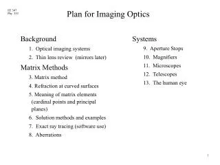
Plan for Imaging Optics. Background 1. Optical imaging systems 2. Thin lens review (mirrors later) Matrix Methods 3. Matrix method 4. Refraction at curved surfaces 5. Meaning of matrix elements (cardinal points and principal planes) 6. Solution methods and examples

Plan for Imaging Optics
E N D
Presentation Transcript
Plan for Imaging Optics Background 1. Optical imaging systems 2. Thin lens review (mirrors later) Matrix Methods 3. Matrix method 4. Refraction at curved surfaces 5. Meaning of matrix elements (cardinal points and principal planes) 6. Solution methods and examples 7. Exact ray tracing (software use) 8. Aberrations • Systems • 9. Aperture Stops • 10. Magnifiers • 11. Microscopes • 12. Telescopes • 13. The human eye
Optical Devices as Systems • Optical imaging, input-output relations. What is an image? • Importance of reference planes • Real vs. Virtual objects and images • Limitations - aberrations, diffraction, scattering • Aspheric surfaces, quadratic surfaces, and spherical surfaces
Image Attributes • Where is an image formed?? All rays leaving an object point (ideally) arrive at a common image point. • Conventions: 1. Light travels in the +x direction 2. R is positive if V is to the left of C 3. a is positive in the +x, +y quadrant 4. Object distances are positive on the left (-x direction), and image distances are positive on the right (+x direction). • How big is the image?? Lateral magnification definition: MT = yi/yo = -si/so • What kind of image is it, real or virtual?
Geometrical Optics Review Sign Conventions Thin lens, Gaussian optics image location and the Lensmaker's eqn. Magnification of image. Summary of general results.
Paraxial Optics Approximation • Paraxial rays make small angles to the system’s optical axis (<10°). • Transverse dimensions are small compared to radii (R’s) of the optical surfaces. • The thickness of a curved interface becomes ≈ 0. • Snell’s law becomes: nq = n’q’ (the angles q become < 10° also). • Skew rays are the same as projections onto axial planes, and only one axial plane is unique. (Only the x-y plane is analyzed, where x is the optical axis).
Matrix method - Ray matrix • Paraxial rays and the paraxial approximation are used: sin q = q, or use only the first term of the expansion. • Define a ray matrix • How is this different from the text? Why? • Output ray in terms of input ray For translation from o to 1 reference planes: y1 = yo + L a1 a1 = ao
Refraction at a Spherical Surface • Use the paraxial form of Snell’s law: n q = n’ q’ n (a+f) = n’ (a’+f) Also use f = y/R so n (a+ y/R) = n’ (a’+ y/R) and solve for n’a’: Where P = optical refracting power of the surface:
Combining Surfaces and Elements • As a ray goes through the system (from left to right), the matrices for the surfaces and propagation distances are multiplied. Matrix multiplication requires them to be ordered from right (first surface) to left (last surface). • Error check: Det[M] = 1 always.
Thick Lenses 1. multiply the matrices from the front to the back vertices. 2. substitute the curved surface powers.
Thin Lenses • For a thin lens t = 0, and yo = y3. In other words, the translation distance is zero, and the ray exits at the same height that it enters the lens. Use the thick lens matrix with t = 0. • Assume: n = n’ then • This is just the lensmaker’s equation. • You can see that two thin lenses sandwiched together give another thin lens with the sum of the two powers, P = P1 + P2.
Special Planes and Cardinal Points 1. Focal planes - first or front focal plane, and second or back focal plane. 2. Principal planes - where rays from focal points appear to bend. H1 and H2 are principal points (where the principal planes cross the axis). 3. Nodal points - rays entering through the first nodal point exit parallel from the second nodal point. 4. Total is 6 cardinal points. For equal indices (in front and in back of the lens), the nodal points are the same as the principal points.
Meaning of Matrix elements #1 • Between any 2 planes: • Left, any ao gives fixed a1 ––> A = 0 and P1 is at f1 • Right,y1 independent of yo ––> D = 0 and P2 is at f2
Meaning of Matrix elements #2 • Conjugate planes = a pair of corresponding object-image planes • All ao from yo go to the same y1 • C = 0 and D = MT (linear magnification) This relationship can be used to find object and image plane locations.
First Problem Solution Method • Finding conjugate planes - object / image locations. 1. Find system matrix between vertex planes. 2. Use translation matrices to translate from vertices to object and image planes. 3. Moi now connects conjugate planes and so C = 0, and D = MT 4. Now solve for the unknown (object distance, image distance, or system variable). 5. If the refractive index is the same at the object and image, then A = 1/MT . (Can be used as a check.)
Meaning of Matrix Elements #3 • a1 independent of yo, thus B = 0 and A = Ma, angular magnification. • B = 0 means the Power is zero or undetermined. This is a “telescopic” system. • A telescope focused at infinity is like this with parallel input and output rays. The angle of the output rays is bigger by the “angular magnification”.
Locating the Principal Planes • Use y2 = y1 for any a1 (left) and To find D = 1 and C = 0. • Use y1 independent of a2 (right) and And also use y2/f = y2P = -a2 to find B = -P and a2 independent of a1 (left) to get A = 1. • So the Matrix is of the form of a thin lens AND of M = 1 conjugate planes!?!
Distance to the Principal Planes 1. Find system matrix between vertex planes (or any pair of planes. 2. Use translation matrices to translate from vertices to H1 and H2 planes. Sign convention is + object left, + image right. 3. MHH now connects principal planes and so C = 0, B = -P, and A = D = 1. 4. Solve for L1 and L2. These are the distances from any 2 planes to the principal planes. Normally n1 and n2 are 1 in air.
Second Problem Solution Method 1. Find the matrix between the vertices (or any other 2 planes) and the distances to the principal planes. 1/f = P = -B • Split the equivalent thin lens in half at the principal planes. 2. Use the thin lens equation as often as needed with so and si measured with respect to the principal planes.
Drawing the Important Rays • Use the cardinal points to construct a ray diagram for an optical system. 1. Rays from the front focal point F1, that go through an object point, exit parallel to the axis at the height that the input ray hits H1. 2. Parallel input rays through an object point, exit through H2 at the same height, go through the back focal point F2, and through the corresponding image point. 3. The undeviated ray comes from an object point, through the nodal point N1 (same as H1), and it exits at N2 parallel to the input ray. It finally intersects the image plane at the image point.
Paraxial Optics Solution Methods 1. One thin lens – use the 1/si + 1/ so = 1/f equation (same for one curved interface - not very useful or common) 2. 2 curved interfaces – use matrices (repeated use of the 1/si + 1/ so equation can result in errors) 2 thin lenses – use matrices or derived equation (in texts) 3. More complex systems – use matrices 4. Mirrors – convert to equivalent lenses 5. Selecting Matrix Method to use: #1 - direct calculation of conjugate (object / image) planes #2 - H (principal) planes, system becomes simple like a single thin lens and you can use the 1/si + 1/ so equation for repeated solution or design
Treatment of Mirrors by “Unfolding” • For plane mirrors, unfold the optical path and do nothing else. The rays are now straight at the mirror plane (see Fig. (c) at right). • Unfolding can be done visualized graphically, or constructed by equal perpendicular distances on opposite sides of the mirror plane. • Curved mirrors are treated by unfolding and adding a thin lens of equivalent power. In these examples, the source point is shown unfolded, not the continuing ray.
Matrix for a Mirror • Use equal angles of incidence and reflection: • Change to angle on right of mirror (a’ changes sign). So that And In air
Aperture Stops to Control Brightness • The “aperture stop” (AS) limits the light that goes through the system from an axial point on the object. • It defines the cone of rays from/to each object/image point. The marginal rays skim the edge of the AS. • The chief ray (from an object point) passes through the center of the entrance and exit pupils and the AS. • You don’t see the aperture stop in the image (except for brightness).
Stops in a Multi-Lens System 1. Find the AS by finding the object that has the smallest angle when imaged to the back or front of the system. 2. Image the AS to the front of the system to find the entrance pupil. 3. Image the AS to the back of the system to find the exit pupil.
Magnifying Glass • Magnification can be referenced to viewing the image at either infinity or at the near point. The first is more common. • The magnified image angle is compared to the angle of the non-magnified object viewed at the near point (as big as you will ever see it with the unaided eye). [Units are cm.]
Microscope • First lens forms a real image (magnified) at that is viewed with the eye lens acting as a simple magnifier. • Magnification is the product of Mt of the objective and M of the eyepiece. You can show that magnification in terms of the feff for the system is [using cm]:
Telescope • Because of infinite object and image distances, matrices will not work to analyze magnification. You can still analyze ray paths with matrices and focusing not at infinity. • Magnification is the ratio of the angles to the image and the object.
Galileo’s Telescope • Magnification is the same formula (eye lens has a negative focal length). • Image is erect, not inverted, and the telescope is shorter. • More difficult to manufacture with the same quality image as with positive focal length lenses.
Types of Telescopes • Unfold the path to show that this has the same form as a refracting telescope. • In(b) the second mirror extends the effective focal length of the first mirror. • In (c) a second intermediate image is formed by the second mirror. • In all cases, the mirrors can be conic sections to reduce aberrations.
Optical Model for the Human Eye • Here the radius of the retina corresponds to a diameter of one inch. Most material (except the lens) is nearly all water, n = 1.33
Another Model of the Eye (from the text) • Models of the eye tend to start with a sphere about 1” in diameter. • The majority of the refracting power is in the first curved surface of the cornea. • For accommodation, muscles squeeze the lens to make it fatter (shorter f.l.).
Analyzing Fans of Rays • From an off-axis object point, two fans of rays are important to analyze as they go in the entrance pupil of the system: 1. Tangential rays (Meridional rays) in the plane containing the axis. 2. Sagittal rays that lie in a plane perpendicular to the tangential rays. • You can also think of filling the aperture with a rectangular array of rays from the object point.
USAF Resolution Chart and Spatial Frequency • Patterns used to test the resolution optical imaging systems. Spatial frequencies are noted in cycles/mm or line-pairs/mm.