Download

1 / 35
350 likes | 621 Views
EPI 5344: Survival Analysis in Epidemiology Confounding and Effect Modification March 25, 2014. Dr. N. Birkett, Department of Epidemiology & Community Medicine, University of Ottawa. Objectives. Review confounding and effect modification (EM) Graphical view of confounding and EM

E N D
EPI 5344:Survival Analysis in EpidemiologyConfounding and Effect ModificationMarch 25, 2014 Dr. N. Birkett, Department of Epidemiology & Community Medicine, University of Ottawa
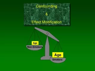
Objectives • Review confounding and effect modification (EM) • Graphical view of confounding and EM • Linear regression model for confounding/EM • How to detect/adjust for confounding in Cox modeling • Effect modification and Cox modeling.
Introduction (1) • In etiological study, interest is on effect of ‘X’ on ‘Y’ • Suppose we have a third variable ‘C’ which explains some of the effect of ‘X’: C X Y • Confounding.
Introduction (2) • A common definition is based on ‘change in estimate of coefficient’ • Estimate the crude OR/RR/etc. (RRcrude) • Estimate OR/RR after adjusting for ‘C’ (RRadj) • If RRadj differs from RRcrude by ‘enough to matter’, we have confounding. • Usually look for 10%+ in RR (or ln(RR)):
Introduction (3) • There is controversy over this definition of confounding. • Pearl and others have shown that, in some situations, an unadjusted estimate for RR can be more valid than an adjusted one. • Argues against using the ‘change in estimate’ method. • This course isn’t the place to explore the debate. • We will use the ‘change in estimate’ approach.
Introduction (4) • Effect Modification • Main interest is relationship of ‘X’ to ‘Y’ • What if a third variable ‘modifies’ that relationship so that it is very different in two or more groups? • Example • RRcrude = 1.7 (1.0-2.4) • RRmale =15.6 (11.0-22.0) **** • RRfemale = 0.4 (0.1-0.6) **** • What is the effect of ‘X’ on ‘Y’?
Introduction (5) • IT DEPENDS! • In men: risk is much higher • In women: risk is much lower • Effect Modification occurs when a third variable defines groups where the relationship differs ‘enough to matter’ • For OR/RR/etc., usually want • Can also look for statistically significant differences between the groups • Tests have low power
Introduction (6) • How do we know if we have either of confounding or effect modification? • There are rules-of-thumb • These are not ‘truth’. • Answer depends on the impact of the results • Does the modification of the OR/RR by a third factor introduce enough difference ‘to matter’? • If so, then confounding/EM • If not, then no confounding/EM
Introduction (7) • This is an empirical/practical approach • Requires knowledge of the scientific field under study • Impact on clinical/scientific/policy decisions • if the HR is 10.0, then an adjustment to 9.0 or 11.0 won’t matter • Some other views • Confounding applies in the ‘population’, not your study. Always matters • Causal modeling • Impact on understanding causal paths as opposed to making practical decisions.
Confounding (1) • Consider this research situation
Age vs. SBP SBP All subjects combined age Now, look at the Rx and control groups separately
Age vs. SBP Control SBP Rx Δ true age Treatment effect is the distance between the lines • It is the same at every age
Assume Rx group is older Control Δ observed Rx Δ true
Assume control group is older Control Δ observed Rx Δ true
Assume groups are same age Control Δ observed Rx Δ true
Assume groups are same age Control Δ observed Rx Δ true
Confounding (2) • We can adjust for confounding by making the age in the two groups ‘the same’ • Design • Matching • RCT • Restriction • Analysis • Graphs are hard to work with, so let’s switch to regression models. • I’ll use linear regression for now
Confounding (3) Cont: yi = B0,cont + B1(age)i Rx: yi = B0,Rx + B1(age)i Note: the slopes are assumed to be the same True effect confounding effect
Confounding (4) True effect confounding effect Confounding = 0 iff Β1=0 OR mean ages are the same
Confounding (5) • How to estimate the Beta’s? • Could do stratified regression (in each treatment group) • Limits your options • Instead, let’s create one regression model which includes both stratified models as sub-models.
Rx Control 0
Confounding (6) • Define zi = 0 if in control group = 1 if in Rx group which can be written as:
Confounding (7) • β2 = adjusted effect of Rx • Can use this model to test hypotheses about adjusted effect, get 95% CI’s, etc.
Confounding (8) • To check for confounding, fit this model with and without ‘age’. • Compare the change in β2from model without age to the model with age • Look for 10% change • Note that this is equivalent to previous ‘rule’ using the logs of the RR/OR/etc.
Now, consider this situation EFFECT MODIFICATION Control SBP Rx age The treatment effect DEPENDS on the age of the subject • Small for low age • Large for high age
Effect Modification (1) • Can also put this into regression models • Key is to note that the slopes aren’t the same. • As before, define: zi = 0 if in control group = 1 if in Rx group
Effect Modification (2) which can be written as: β3≠0 Effect Modification
Use in Cox • Linear regression model is called: • Parallel line analysis • Extends easily to Cox models. • Replace ‘y’ by ‘ln(HR)’ • Remember, no intercept for the Cox model (contained in h0(t)) If there is no EM, we get: Effect of ‘z’ adjusted for ‘x’ Compare to model with only ‘z’ to check confounding
SAS code (1) TO CHECK FOR EM: proc phreg data=njb1; class z/param=ref ref=first; model time*cens(0)=x z x*z; run; Look at the ‘Beta’ for ‘x*z’ to check for EM.
SAS code (2) If there is no EM, run two more models to check for confounding. ADJUSTED MODEL proc phreg data=njb1; class z/param=ref ref=first; model time*cens(0)=x z; run; CRUDE MODEL proc phreg data=njb1; class z/param=ref ref=first; model time*cens(0)=z; run; Compare the ‘Beta’ for ‘z’ in these two models
SAS code (3) • What if ‘z’ has more than 2 levels? • Can use the same code • Effect Modification • Use the likelihood ratio test (-2Δlog(L)) • Available directly in SAS output • Confounding • Need to consider possible confounding for each level of ‘z’ • Overall decision to adjust for ‘x’ depends on presence of any confounding.
Rx effect when there is EM (1) • Our Cox model is: • What is the effect of ‘z’ on the HR? • If there were no interaction, can just use exp(β2) • But, this is not appropriate with interaction:
Rx effect when there is EM (2) • There is no single treatment effect. • Depends on value of EM variable • Need to present effect estimates in a graph or table (or formula)