Download
1 / 56
560 likes | 702 Views
University of St Andrews. School of Physics and Astronomy. Thermodynamics of phase formation in Sr 3 Ru 2 O 7. Andy Mackenzie. University of St Andrews, UK. PITP Toronto 2008. University of St Andrews. Collaborators. M. Allan 1 , F. Baumberger 1 , R.A. Borzi 1 , J.C. Davis 1,3,4 ,

E N D
University of St Andrews School of Physics and Astronomy Thermodynamics of phase formation in Sr3Ru2O7 Andy Mackenzie University of St Andrews, UK PITP Toronto 2008
University of St Andrews Collaborators M. Allan1, F. Baumberger1, R.A. Borzi1, J.C. Davis1,3,4, J. Farrell1,S.A. Grigera1, J. Lee4, Y. Maeno5, J.F. Mercure1, R.S. Perry1,2, A. Rost1,Z.X. Shen6, A. Tamai1, A. Wang3 1 University of St Andrews; 2 University of Edinburgh; 3 Cornell University; 4 Brookhaven National Laboratory 5 Kyoto University; 6 Stanford University
Contents 1. Introduction – materials and terminology 2. Metamagnetic quantum criticality and low-frequency dynamical susceptibility in slightly dirty Sr3Ru2O7. 3. Phase formation in ultra-pure Sr3Ru2O7 4. Magnetocaloric effect as a probe of the ‘entropic landscape’ 5. Spectroscopic imaging of conductance oscillations around scattering centres: a dynamics-to-statics transducer. 6. Conclusions
M H H Metamagnets and the vapour-liquid transition Mapping between both systems P, T, r H, T, M T T Critical end-point vapour 1st order liquid P H
Metamagnets and Quantum Critical Points Important difference with water: The transition can be tuned to T=0. Large majority of real itinerant metamagnets are first order at T = 0 even after best effort to tune. See e.g. T.Goto et al., Physica B 300, 167 (2001) T Critical end-point 1st order h u
c-axis (90) 1 4 0 0 1 2 0 0 q ] K m 1 0 0 0 [ e r u 8 0 0 t a r e p 6 0 0 m e T 4 0 0 8 2 0 0 ] 7 a l s 0 e 0 t [ 6 2 0 d l e 4 0 a i n g F l 6 0 e f r o 5 m 8 0 a b [ d e 1 0 0 g r e e s ] Experimental phase diagram of “clean” Sr3Ru2O7 T* inferred from maximum in real part of a.c. susceptibility Plane defined by maxima of imaginary part Quantum critical end-point S.A. Grigera, R.A. Borzi, A.P. Mackenzie, S.R. Julian, R.S. Perry & Y. Maeno, Phys. Rev. B 67, 214427 (2003).
Constructing the experimental phase diagram 1.2 1.2 1.2 1.2 7.9 6.5 7.9 6.5 0.8 0.8 0.8 0.8 5.5 6.4 6.4 5.5 T (K) T (K) T (K) T (K) 0.4 0.4 0.4 0.4 Field (tesla) Field (tesla) Field (tesla) Field (tesla) 0.0 0.0 0.0 0.0 4.9 4.5 4.9 4.5 T* = 1.05K q = 40° x 10 T* = 1.25K q = 0 (H // ab) x 10
1.2 1.2 1.2 1.2 8.5 7.5 7.5 8.5 0.8 0.8 0.8 0.8 7.5 7.5 6.5 6.5 T (K) T (K) T (K) T (K) 0.4 0.4 0.4 0.4 Field (tesla) Field (tesla) Field (tesla) Field (tesla) 0.0 0.0 0.0 0.0 6.5 5.5 5.5 6.5 q = 90° (H // c) T* < 0.1K x 10 No evidence of first-order behaviour for H // c q = 60° x 10 T* = 0.55K x 0.5
Evidence for very slow dynamics 4 cmax (10-6 m3/mol Ru) 2 1.2 1.2 7.9 7.9 0.8 0.8 6.4 6.4 0 T (K) T (K) 0.4 0.4 1 2 3 Field (tesla) Field (tesla) 0.0 0.0 4.9 4.9 f (kHz) q = 0 (H // ab) Why are the global maxima so weak? q = 40° Large changes at amazingly low frequency
Approach to criticality ‘cut off’ by a new phase in highest purity samples (l ~ 3000 Å) - Resistivity: dr/dH and d2r/dT2 - Susceptibility: c’ and c’’ - Magnetostriction:l(H) S.A.Grigera et al., Science 306, 1154 (2004) - Magnetisation 1.2 0.8 P. Gegenwart et al., Phys. Rev. Lett. 96, 136402 (2006) T(K) 0.4 R.A. Borzi et al., Science 315, 214 (2007) 0 7.7 7.9 8.1 8.3 oH (T) Phase lines bound a region with pronounced resistive anisotropy: ‘electronic nematic’ properties
The H-T Phase diagram “The wrong shape” usually: “dome” 1.2 0.8 T(K) 0.4 S> S< here: “muffin” 0 7.7 7.9 8.1 8.3 oH (T) first order phase trasitions? -> Clausius-Clapeyron S inside bigger than S outside
How to “measure the entropy” H Entropy 1 H 2 DT S DS T T 2 1 Temperature → DT > 0 DS < 0
Our experimental setup (Andreas Rost) Kevlar Strings (35 @ 17μm) Thermometer (Resistor) Silver Platform with sample on other side High level of control possible via tunable thermal link; easy system to model. CuBe Springs Copper Ring 2 cm
T [mk] H [T] Sample raw Magnetocaloric Effect data from Sr3Ru2O7 Under fully adiabatic conditions Sharper features associated with first order transitions ‘Signs’ of changes confirm that entropy is higher between the two first order transitions than outside them. Metamagnetic crossover seen in susceptibility
Magnetocaloric quantum oscillations T=150mK 1 T [mK] 0 ΔT [mK] -1 8.5 9 9.5 10 10.5 11 11.5 μ0H [T] μ0H [T] Measurement noise level: 25 μK / √Hz
Magnetocaloric quantum oscillations T=150mK 1 ΔT [mK] T [mK] 0 -1 0.09 0.1 0.11 μ0H [T] 1/μ0H [T-1] Measurement noise level: 25 μK / √Hz
Preliminary conclusions from magnetocaloric effect (MCE) work on Sr3Ru2O7
Preliminary conclusions from magnetocaloric effect (MCE) work on Sr3Ru2O7 • MCE confirms our prior identification of first-order lines as equilibrium phase transitions • Entropy is indeed higher between the lines than either side of them. • ‘Phase’ seems to be characterised by ‘quenching’ of
Taking the next step: the ‘entropic landscape’ T [K] μ0H [T]
Taking the next step: the ‘entropic landscape’ S/T [J/mol K2] 0.27 0.22 0.17 0.12 T [K] μ0H [T]
Taking the next step: the ‘entropic landscape’ S/T [J/mol K2] 0.27 0.22 0.17 T [K] 0.12 T [K] μ0H [T] μ0H [T]
Taking the next step: the ‘entropic landscape’ S/T [J/mol K2] 0.27 0.22 0.17 0.17 T [K] 0.12 0.12 T [K] μ0H [T] μ0H [T]
Taking the next step: the ‘entropic landscape’ S/T [J/mol K2] 0.27 0.22 0.17 T [K] 0.12 T [K] μ0H [T] μ0H [T]
Taking the next step: the ‘entropic landscape’ S/T [J/mol K2] 0.27 T [K] 0.22 0.17 T [K] 0.12 μ0H [T] μ0H [T]
Power Law Fit To Specifc Heat Fitequation data 0.1 fitted curve 0.08 Fitrange 5 T to 7.1 T Resulting Parameters a = 0.004(1) b= -0.99(5) c = -0.012(2) 0.06 (C(H)-C(5T))/ T 0.04 0.02 0 3.5 4 4.5 5 5.5 6 6.5 7 7.5 8 8.5 Field [T]
e Spatially resolved conductance oscillations around scattering centres: a dynamics–to–statics transducer q > 2kF e = eF q = 2kF q < 2kF -kF k kF G dHvA and STM QPI and ARPES: Fermi velocities in Sr3Ru2O7 of 10 km/s and below: suppressed from LDA values by at least a factor of 20: direct observation of d-shell heavy fermions.
Conclusions • Sr3Ru2O7 can be tuned towards a quantum critical metamagnetic transition. • If this is done in ultra-pure crystals (mfp > 3000Å) a new phase forms before the quantum critical point is reached. • Material with slight disorder shows strongly frequency-dependent low T susceptibility; situation in pure material still needs to be investigated. • The magnetocaloric effect, if measured with care in a calibrated system, can give a comprehensive picture of the entropy evolution near QCPs.
S/T [J/mol K2] T [K] μ0H [T]
0.09 0.05 0 T = 600 mK ΔS (J/K) 7 7.5 8 8.5 Field (T)
Consider the ferromagnetic superconductor URhGe Metamagnetic transition due to spin reorientation deep in ferromagnetic state Superconductivity at low T, B Metamagnetic QCP? D. Aoki, I Sheikin, J Flouquet & A. Huxley, Nature 413, 613 (2001)
In URhGe the new phase in the vicinity of the metamagnetic QCP is superconducting Re-entrant superconductivity! F. Lévy, I. Sheikin, V. Hardy & A. Huxley, Science 309, 1343 (2005). Perspective: A.P. Mackenzie & S.A. Grigera, ibid p. 1330
Potentially more than ‘just’ interesting basic science: 25 T insufficient to destroy superconductivity although Tc < 0.5 K! F. Lévy, I. Sheikin & A. Huxley, Nature Physics 3, 461 (2007)
Pronounced resistive anisotropy in a region of phase space bounded by low T 1st order phase transitions r T = 100 mK J H H J J H J //H R.A. Borzi, S.A. Grigera, J. Farrell, R.S. Perry, S. Lister, S.L. Lee, D.A. Tennant, Y. Maeno & A.P. Mackenzie, Science 315, 214 (2007)
T = 100 mK ac (arb. Units) (cm)
Example of magneto-thermal oscillation with field aligned to c-axis H [T]
University of St Andrews Low-T susceptibility is remarkably isotropic and T-independent: strongly enhanced Pauli paramagnet on verge of ferromagnetism? S.I. Ikeda, Y. Maeno, S. Nakatsuji, M. Kosaka and Y. Uwatoko, Phys. Rev. B 62, R6089 (2000). Basic bulk properties of Sr3Ru2O7 At low temperature and low applied magnetic field, it is an anisotropic Fermi liquid (rc / rab 100). Structure chi(T) and refto Shinichi etc.
Ruthenates: electronic structure considerations d shell tet. cryst. field filling & hybridisation
Ruthenates: electronic structure considerations Cu2+ 3d9 d shell tet. cryst. field filling & hybridisation
Ruthenates: electronic structure considerations Ru4+ 4d4 d shell tet. cryst. field filling & hybridisation
Intermediate Report 23rd September 2008
Entropy Change 0.1 0.05 0 -0.05 -0.1 Entropy change (S(H)-S(5T))/ T -0.15 -0.2 -0.25 -0.3 4 5 6 7 8 9 10 11 12 13 Field [T] • (S(H)-S(5T))/T as a function of H • Different temperatures are offset • for clarity Decreasing T
Entropy Surface (S(H)-S(5T))/T [J / mol K^2] T [K] H [T]
Entropy Surface (S(H)-S(5T))/T [J / mol K^2] T [K] H [T]
Entropy Surface T [k] H [T]
Entropy Change 0.1 0.05 0 -0.05 -0.1 Entropy change (S(H)-S(5T))/ T -0.15 -0.2 -0.25 -0.3 4 5 6 7 8 9 10 11 12 13 Field [T] • (S(H)-S(5T))/T as a function of H • Different temperatures are offset • for clarity Decreasing T
Entropy Change 0.1 0.05 0 For better comparison I will choose 4 traces at T= (230mK, 400mK,900mK,1450mK) -0.05 -0.1 Entropy change (S(H)-S(5T))/ T -0.15 -0.2 -0.25 -0.3 4 5 6 7 8 9 10 11 12 13 Field [T]
Entropy Change 0.1 0.05 0 -0.05 -0.1 -0.15 -0.2 -0.25 -0.3 4 5 6 7 8 9 10 11 12 13 230mK For better comparison I will choose 4 traces at T= (230mK, 400mK,900mK,1450mK) 400mK Entropy change (S(H)-S(5T))/ T 900mK 1450mK Field [T]
Entropy Change 0.1 0.1 0.05 0 0.08 -0.05 0.06 -0.1 -0.15 0.04 -0.2 0.02 -0.25 -0.3 0 4 5 6 7 8 9 10 11 12 13 4 5 6 7 8 9 Entropy change (S(H)-S(5T))/ T Field [T] Field [T] On the right these curves are plot without offset