Fast Temporal Calibration Methodology for Tracked Ultrasound: A Robust Approach
This study presents a novel, fully automatic temporal calibration methodology for tracked ultrasound (US) systems, addressing the misalignment between imaging and tracking timestamps. By utilizing the RANSAC algorithm, the method accurately aligns tracker and image position signals through time offset computation. Evaluated on 200 diverse US sequences, the algorithm demonstrated precise calibration, achieving standard deviations of less than 5 ms for consistent imaging parameters. The freely available code contributes significantly to the ultrasound research community, promoting improved accuracy in tracked ultrasound applications.

Fast Temporal Calibration Methodology for Tracked Ultrasound: A Robust Approach
E N D
Presentation Transcript
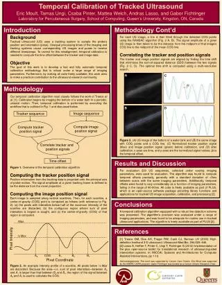
Temporal Calibration of Tracked Ultrasound Eric Moult, TamasUngi, Csaba Pinter, Mattea Welch, Andras Lasso, and Gabor Fichtinger Laboratory for Percutaneous Surgery, School of Computing, Queen’s University, Kingston, ON, Canada Tracker sequence Compute image position signal Compute tracker position signal Introduction Methodology Cont’d Correlate tracker and position signals Background Tracked ultrasound (US) uses a tracking system to sample the probe’s position and orientation (pose). Unequal processing times of the imaging and tracking systems cause corresponding US images and poses to receive different timestamps. To correct for this misalignment, temporal calibration is needed to compute the time offset between the tracker and image data. Objective The goal of this work is to develop a fastand fully automatic temporal calibration methodology that is robust under a large range of imaging parameters. Furthermore, by making all code freely available, this work aims to make a practical contribution to the ultrasound research community. For each US image, a line is then fitted through the detected COG points using the RANSAC algorithm (Fig. 3 A, B). The signal amplitude of a given US image is then taken to be the distance from the midpoint of that image’s COG line to the midpoint of the mean COG line. Correlating the tracker and position signals The tracker and image position signals are aligned by finding the time shift that minimizes the sum-of-squared distance (SDD) between the two signals (Fig. 3 C, D). The optimal time shift is computed using a multi-resolution search. Figure 3. (A) US image of the bottom of a water tank and (B)the same image with COG points and a COG line. (C) Normalized tracker position signal (blue) and image position signal (green) before calibration, and (D) after calibration. x-axes are time, and y-axes are the normalized signal values; Δt is the temporal offset. Time offset A C Methodology Our temporal calibration algorithm most closely follows the work of Treeceet al. [1].Calibration begins by imaging the bottom of a water bath in a periodic, uniaxial motion. Then, temporal calibration is performed by executing the workflow that is outlined in Fig. 1 and discussed below. Figure 1. Overview of the temporal calibration algorithm Computing the tracker position signal Position information from the tracking data is projected onto the principal axis of probe motion. The signal amplitude at a given tracking frame is defined to be the distance from the mean projection. Computing the image position signal Each image is sampled along vertical scanlines. Then, for each scanline, a center-of-gravity (COG) point is computed as follows (with reference to Fig. 2): (a) the pixels with intensities below half of the maximum intensity of the scanline are discarded, (b) the contiguous region whose sum of pixel intensities is largest is sought, and (c) the center-of-gravity (COG) of that region is computed. Figure 2. An example intensity profile of a scanline. All pixels below ½ Max are discarded. Because the area—i.e. sum of pixel intensities—between A0 and A1is larger than that between B0and B1,the region of the signal between A0 and A1is used to calculate the COG. B D Image sequence Image sequence Results and Discussion For evaluation 200 US sequences, collected under varying imaging parameters, were used for evaluation. The algorithm was found to compute temporal offsets precisely, generally with a standard deviation of <5ms between scans with the same imaging parameters. Additionally, temporal offsets were found to vary considerably as a function of imaging parameters, falling in the range of 40-90ms. All code is freely available as part of PLUS, which is an open-source software package providing library functions and applications for tracked US image acquisition, calibration, and processing [2]. Conclusions A temporal calibration algorithm equipped with a robust line detection scheme was presented. The algorithm’s precision was evaluated under a range of imaging parameters, and was found to be adequate for routine use in tracked ultrasound applications. The algorithm is freely available as part of PLUS[2]. Max References ½ Max [1] Treece GM, Gee AH, Prager RW, Cash CJ, Berman LH (2003) High-definition freehand 3-D ultrasound. Ultrasound Med Bio. 294:529–546. [2] Lasso A, Heffter T, Pinter C, Ungi T, Fichtinger G (2012) Implementation of the plus open-source toolkit for translational research of ultrasound-guided intervention systems. In: MICCAI, Systems and Architectures for Computer Assisted Interventions, pp 1-12. Acknowledgements: This work was supported by Cancer Care Ontario. Eric Moult was supported by the NSERC USRA program. Gabor Fichtinger was funded as a Cancer Ontario Research Chair. Pixel Intensity B0 B1 A1 A0 COG Pixel Coordinate