Download
1 / 14
140 likes | 221 Views
Proposed Dissimilarity Measure. We chose the SDF as our shape descriptor because: Convergence condition of gradient descent methods is satisfied (Huang et al PAMI’06). Invariance to rotations and translations. Ability to handle topological changes. Its relative simplicity.

E N D
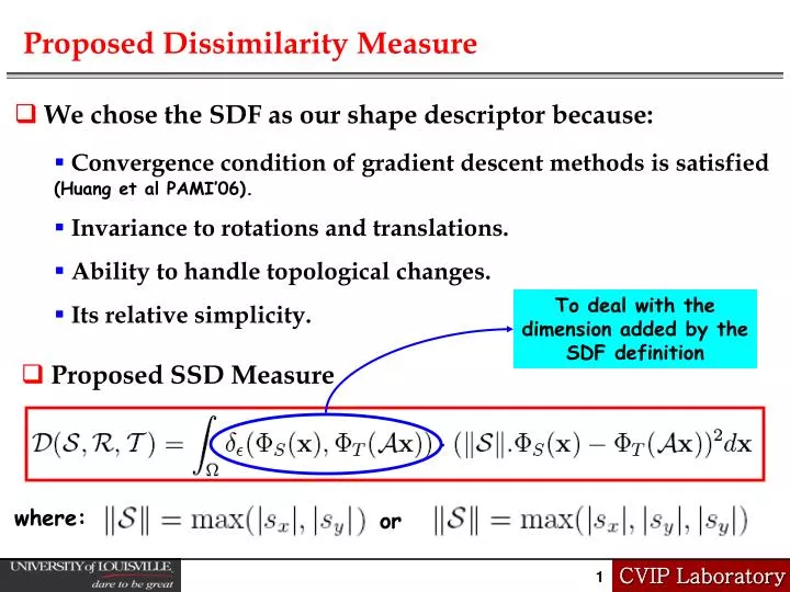
Proposed Dissimilarity Measure • We chose the SDF as our shape descriptor because: • Convergence condition of gradient descent methods is satisfied(Huang et al PAMI’06). • Invariance to rotations and translations. • Ability to handle topological changes. • Its relative simplicity. To deal with the dimension added by the SDF definition • Proposed SSD Measure where: or
Convexity of the proposed SSD measure • Empirical Evaluation (2D case): • Pick a shape: • Fix 3 parameters and vary the remaining 2. • The ranges of the 2 unknown parameters are uniformly quantized using 100 samples: • Convexity in full dimensionality is not guaranteed
Euler Lagrange Equations • For each parameter where: • Implementation consideration: different time steps may need to be used for different parameters
Comparisons with the other models Initial position Isotropic scale-based model VDF-based model 208.67 sec 300.57 sec 141.26 sec 221.35sec Our results 139.67 sec 206.82sec 180.68sec 102.23sec
More comparisons Initial position Isotropic scale-based model VDF-based model 538.67sec 271.57 sec 263.69 sec 219.87 sec 296.67sec 157.76 sec 147.20 sec Our results 169.77 sec
Recovered parameters • GT: Ground truth • M1: Our model • M2:VDF-model • M3: Homogeneous scale-based model
Model shape variations using PCA Align Shapes Application: Statistical modeling of shapes Shape Model = Mean Shape + Basic Variations Implicit Rep. Training data
Before alignments Overlap After alignments Overlap Alignments Goal: Establish correspondences among shapes over the training set
Qualitative Evaluation • Correlation Coefficient
Modeling shape variations using PCA • Compute the mean of the aligned data and mean offsets and • SVD of covariance matrix with • New shape, within the variance observed in training set, can be approximated chose k s.t.
First four principal modes Mode 1 Mode 2 Mode 3 Mode 4
Application: Shape-based segmentation • Generate an Active Shape Model (ASM) and use it to locate objects in hard to segment images (Cootes and Taylor’95) Isotropic scale-based model Our model