Download
1 / 13
130 likes | 279 Views
Lecture 4: The Atmosphere & Its Circulation Part 2. Fluid Convection. Schematic of shallow convection in a fluid , such as water, triggered by warming from below and/or cooling from above.

E N D
Fluid Convection Schematic of shallow convection in a fluid, such as water, triggered by warming from below and/or cooling from above. When a fluid such as water is heated from below (or cooled from above), it develops overturning motions. This seems obvious. A thought experiment: consider the shallow, horizontally infinite fluid shown in Figure above. Let the heating be applied uniformly at the base; then we may expect the fluid to have a horizontally uniform temperature, so T = T(z) only. The fluid will be top-heavy: warmer and therefore lighter fluid below cold, dense fluid above. The situation does not contradict hydrostacy: ∂p/∂z = -gρ. BUT, 1. Why do motions develop when we can have hydrostatic equilibrium, with no net forces? 2. Why are the motions can become horizontally inhomogeneous when the heating is horizontally uniform? Answer: because the “top-heavy” state of the fluid is unstable
Understanding instability x Consider point “A” or “B” – is the state of the ball stable? When perturbed, if the ball moves farther and farther from its original position, then unstbale; otherwise the system is stable. For small distances x from “A” (or “B”), acceleration is d2x/dt2;thereforealong the slope,d2x/dt2=−gdh/dx = −g(d2h/dx2)Ax(Taylor expansion about “A” where dh/dx = 0) Solution is: x ~ exp(.t) where = [−g(d2h/dx2)A]1/2 Thus: at “A” where (d2h/dx2) < 0, the solution has an exponentially growing part, indicating instability; at “B” the solution is oscillatory, but stable. When the ball is perturbed from the crest (top of hill) it moves downslope, its potential energy decreases and its kinetic energy increases– unstable. In the valley, by contrast, one must keep on supplying potential energy to push the ball up, for otherwise it will sink back to the valley – stable. Stability and instability of a ball on a curved surface.
Buoyancy in water – an incompressible fluid A parcel of light, buoyant fluid surrounded by resting, homogeneous, heavier fluid in hydrostatic balance, ∂p/∂z = -gρ. The fluid above points A1, A, and A2 has the same density, and hence, by hydrostacy, pressures at the A points are all the same. But the pressure at B is lower than at B1 or B2 because the column of fluid above B is lighter. There is thus a pressure gradient force which drives fluid inwards toward B (blue arrows), tending to equalize the pressure along B1BB2. The pressure at B will tend to increase, forcing the light fluid upward, as indicated schematically by the red arrows. The acceleration or buoyancy of the parcel of fluid is b = -gρ/ρP, ρ= ρP - ρE i.e. parcel minus environment densities.
Stability of a parcel in water Consider a fluid parcel initially at z1in an environment whose density is ρ(z) (see Figure on right). The parcel’s density ρ1 = ρ(z1), is the same as its environment at height z1. The parcel is now displaced without loosing or gaining heat (i.e. adiabatically), and also without expanding or contracting (incompressible), a small vertical distance to z2 = z1+ δz, where the new environment density is: ρE= ρ(z2) ρ1 + (dρ/dz)Eδz. The parcel’s buoyancy is then: b = -g(ρ1- ρE)/ρ1 = g(dρ/dz)Eδz /ρ1. Therefore, if (dρ/dz)E> 0 parcel keeps rising unstable (dρ/dz)E= 0 parcel stays neutrally stable (dρ/dz)E< 0 parcel returns stable An incompressible liquid is unstable if density increases with height (in the absence of viscous and diffusive effects)
Homework: stability using potential energy (PE) argument Consider again the Figure on right. Imagine that the 2 fluid parcels (“1” and “2”) exchange their positions. Before the exchange, the PE (focusing on these 2 parcels) is: PEbefore = g (ρ1z1 + ρ2z2) After the exchange: PEafter= g (ρ1z2+ ρ2z1). Show that: PE = −g (ρ2 − ρ1) (z2 − z1) Then show: PE = -g(dρ/dz)E(z2– z1)2 . Then deduce and explain the stabilityand instability of the system based on the sign of PE.
Laboratory experiment of convection Parcels overshoot Gravity waves 32 oC 14 oC c) (a) A sketch of the laboratory apparatus used to study convection. A stable stratification is set up in a 50cm × 50 cm × 50 cm tank by slowly filling it up with water whose temperature is slowly increased with time. This is done using (1) a mixer, which mixes hot and cold water together, and (2) a diffuser, which floats on the top of the rising water and ensures that the warming water floats on the top without generating turbulence. Using the hot and cold water supply we can achieve a temperature difference of 20◦C over the depth of the tank. The temperature profile is measured and recorded using thermometers attached to the side of the tank. Heating at the base is supplied by a heating pad. The motion of the fluid is made visible by sprinkling a very small amount of potassium permanganate (which turns the water pink) after the stable stratification has been set up and just before turning on the heating pad. Convection carries heat from the heating pad into the body of the fluid, distributing it over the convection layer much like convection carries heat away from the Earth’s surface. (b) Schematic of evolving convective boundary layer heated from below. The initial linear temperature profile is TE. The convection layer is mixed by convection to a uniform temperature. Fluid parcels overshoot into the stable stratification above, creating the inversion evident in (c). Both the temperature of the convection layer and its depth slowly increase with time.
Laboratory experiment: more discussions Heating starts 5 4 3 2 1 Parcels overshoot Gravity waves 5 Heating 4 3 Left: Parcels overshoot the neutrally buoyant level, brush the stratified layer above, produce gravity waves, then sink back into the convective layer beneath Right: Temperature time series measured by five thermometers spanning the depth of the fluid at equal intervals shown on left. The lowest thermometer is close to the heating pad. We see that the ambient fluid initially has a roughly constant stratification, somewhat higher near the top than in the body of the fluid. The heating pad was switched on at t = 150 sec. Note how all the readings converge onto one line as the well mixed convection layer deepens over time. 2 1
Appendix: Law of vertical heat transport Heat flux up = 0.5*ρrefcp(T+ T)wc H = heat flux = amount of heat transported across unit volume in unit time = (ρcpT)w (For water: cp= 4000 J kg−1 K−1) Cooler: T Heat flux down = 0.5*ρrefcpwcT Warmer: T+ T So, net heat flux, averaged horizontally, is H = (flux up – flux down) = 0.5*ρrefcpwcT. As light fluid rises and dense fluid sinks, PE = −g (ρ2 − ρ1) (z2 − z1) = -gρz KE = 3 × 0.5*ρrefwc2 (assuming isotropic motion – same in all 3 directions) So, wc2 (2/3).αgzT i.e. H= 0.5*ρrefcpwcT 0.5*ρrefcp[(2/3).αgz]1/2T3/2 . In the laboratory experiment, the heating coil provides H = 4000 W m−2. If the convection penetrates over a vertical scale z = 0.2 m, then using α = 2 × 10⁻⁴ K−1 and cp= 4000 J kg−1 K−1, we obtain: T 0.1K and wc 0.5 cm s−1.
Stability of a dry & compressibleatmosphere The real atmosphere is compressible, so that e.g. an air parcel can expand when experiencing less pressure, i.e. its density not only depends on T, but also on pressure p. As the parcel rises, it moves into an environment of lower pressure. The parcel will adjust to this pressure; in doing so it will expand, doing work on its surroundings, and thus cool. If after the parcel cools, it is still warmer than the new surrounding at the greater height, then the parcel will keep on rising, and the atmosphere is unstable. Thus for convection to occur, it is not enough for the atmosphere’s temperature to decrease with height, it must decrease faster than the rate at which an air parcel’s temperature decreases with height as the parcel expands – this rate is called the Dry Adiabatic Lapse Rate = -g/cp10 K km−1, using cp= 1005 J kg−1K−1 for air. In the tropic, the atmosphere has dT/dz-4.6K km−1, so is actually stable to dry convection. It is the release of latent heat which makes the air parcel unstable: Moist Adiabatic Lapse Rate 3K km−1.
10 km 5 km 200 K 250 K 300 K A schematic of tropospheric temperature profiles showing the dry adiabat, a typical wet adiabat, and a typical observed profile. Note that the dry adiabatic ascent of a parcel is typically cooler than the surroundings at all levels, whereas the wet adiabat is warmer up to about 10 km. The wet and dry lapse rates are close to one another in the upper troposphere, where the atmosphere is rather dry.
Outgoing longwave radiation (OLR: contour interval 20 W m−2) averaged over the year. Note the high values over the subtropics and low values over the three wet regions on the equator: Indonesia, Amazonia, and equatorial Africa