Download
1 / 89
900 likes | 1.36k Views
Computational methods in phylogenetic analysis. Tutorial at CSB 2004 Tandy Warnow. Reconstructing the “Tree” of Life. Handling large datasets: millions of species. Phylogenetic Inference. Hard optimization problems (e.g. MP, ML) Better heuristics

E N D
Computational methods in phylogenetic analysis Tutorial at CSB 2004 Tandy Warnow
Reconstructing the “Tree” of Life Handling large datasets: millions of species
Phylogenetic Inference • Hard optimization problems (e.g. MP, ML) • Better heuristics • Better approximations/lower bounds Relationship between quality of optimization criterion and topological accuracy
Phylogenetic Inference, cont. • Bayesian inference • Whole Genome Rearrangements • Reticulate evolution • Processing sets of trees: compact representations and consensus methods • Supertree methods • Statistical issues with respect to stochastic models of evolution (e.g., “fast converging methods”) • Multiple sequence alignment
Major challenge: MP and ML • Maximum Parsimony (MP) and Maximum Likelihood (ML) remain the methods of choice for most systematists • The main challenge here is to make it possible to obtain good solutions to MP or ML in reasonable time periods on large datasets
Outline • Part I (Basics): 40 minutes • Part II (Models of evolution): 20 min. • Part III (Distance-based methods): 30 min. • Part IV (Maximum Parsimony): 30 min. • Part V (Maximum Likelihood): 15 minutes • Part VI (Open problems/research directions): 30 minutes
Part I: Basics (40 minutes) Questions: • What is a phylogeny? • What data are used? • What are the most popular methods? • What is meant by “accuracy”, and how is it measured? • What is involved in a phylogenetic analysis?
Phylogeny From the Tree of the Life Website,University of Arizona Orangutan Human Gorilla Chimpanzee
Data • Biomolecular sequences: DNA, RNA, amino acid, in a multiple alignment • Molecular markers (e.g., SNPs, RFLPs, etc.) • Morphology • Gene order and content These are “character data”: each character is a function mapping the set of taxa to distinct states (equivalence classes), with evolution modelled as a process that changes the state of a character
-3 mil yrs AAGACTT AAGACTT -2 mil yrs AAGGCCT AAGGCCT AAGGCCT AAGGCCT TGGACTT TGGACTT TGGACTT TGGACTT -1 mil yrs AGGGCAT AGGGCAT AGGGCAT TAGCCCT TAGCCCT TAGCCCT AGCACTT AGCACTT AGCACTT today AGGGCAT TAGCCCA TAGACTT AGCACAA AGCGCTT AGGGCAT TAGCCCA TAGACTT AGCACAA AGCGCTT DNA Sequence Evolution
Phylogeny Problem U V W X Y AGGGCAT TAGCCCA TAGACTT TGCACAA TGCGCTT X U Y V W
Phylogenetic Analyses • Step 1: Gather sequence data, and estimate the multiple alignment of the sequences. • Step 2: Reconstruct trees on the data. (This can result in many trees.) • Step 3: Apply consensus methods to the set of trees to figure out what is reliable.
Reconstruction methods • Much software exists, most of which attempt to solve one of two major optimization criteria: Maximum Parsimony and Maximum Likelihood. The most frequently used software package is PAUP*, which contains many different heuristics. • Methods for phylogeny reconstruction are evaluated primarily in simulation studies, based upon stochastic models of evolution.
The Jukes-Cantor model of site evolution • Each “site” is a position in a sequence • The state (i.e., nucleotide) of each site at the root is random • The sites evolve independently and identically (i.i.d.) • If the site changes its state on an edge, it changes with equal probability to the other states • For every edge e, p(e) is defined, which is the probability of change for a random site on the edge e.
Methods for phylogenetic inference • Polynomial time methods, mostly based upon estimating evolutionary distances between sequences, and then using them to construct a tree with edge lengths • Heuristics for hard optimization problems (such as maximum parsimony and maximum likelihood) • Bayesian MCMC methods
Standard problem: Maximum Parsimony (Hamming distance Steiner Tree) • Input: Set S of n aligned sequences of length k • Output: A phylogenetic tree T • leaf-labeled by sequences in S • additional sequences of length k labeling the internal nodes of T such that is minimized.
Maximum parsimony (example) • Input: Four sequences • ACT • ACA • GTT • GTA • Question: which of the three trees has the best MP scores?
Maximum Parsimony ACT ACT ACA GTA GTT GTT ACA GTA GTA ACA ACT GTT
Maximum Parsimony ACT ACT ACA GTA GTT GTA ACA ACT 2 1 1 3 3 2 GTT GTT ACA GTA MP score = 7 MP score = 5 GTA ACA ACA GTA 2 1 1 ACT GTT MP score = 4 Optimal MP tree
Optimal labeling can be computed in linear time O(nk) GTA ACA ACA GTA 2 1 1 ACT GTT MP score = 4 Finding the optimal MP tree is NP-hard Maximum Parsimony: computational complexity
Maximum Likelihood (ML) • Given: stochastic model of sequence evolution (e.g. Jukes-Cantor) and a set S of sequences • Objective: Find tree T and probabilities p(e) of substitution on each edge, to maximize the probability of the data. Preferred by some systematists, but even harder than MP in practice.
Bayesian MCMC • Assumes a model of evolution (e.g., Jukes-Cantor) • The basic algorithmic approach is a random walk through the space of model trees, with the probability of the data on the model tree determining whether the proposed new model tree is accepted or rejected. • Statistics on the set of trees visited after “burn-in” constitute the output.
Performance criteria for phylogeny reconstruction methods • Speed • Space • Optimality criterion accuracy • “Topological accuracy” (specifically statistical consistency, convergence rate, and performance on finite data) These criteria can be evaluated on real or simulated data.
Evaluating MP heuristics with respect to MP scores Fake study Performance of Heuristic 1 MP score of best trees Performance of Heuristic 2 Time
Quantifying Topological Error FN FN: false negative (missing edge) FP: false positive (incorrect edge) 50% error rate FP
Statistical performance issues • Statistical consistency: an estimation method is statistically consistent under a model if the probability that the method returns the true tree goes to 1 as the sequence length goes to infinity • Convergence rate: the amount of data that a method needs to return the true tree with high probability, as a function of the model tree
Practice • In practice, most systematic biologists use either MP or ML on small datasets, and MP or MCMC methods on moderate to large datasets • Distance-based methods (such as neighbor joining) are used by some, but are not considered as reliable as these other approaches.
Major challenges • The main challenge here is to make it possible to obtain good solutions to MP or ML in reasonable time periods on large datasets • MCMC methods are increasingly used (often as a surrogate for a decent ML analysis), but it is not clear how to evaluate MCMC methods
Part II: Models of evolution (20 minutes) • Site evolution models • Variation across sites • Statistical performance issues: statistical identifiability, statistical consistency, convergence rates • Special issues: molecular clock, no-common-mechanism
The Jukes-Cantor model of site evolution • Each “site” is a position in a sequence • The state (i.e., nucleotide) of each site at the root is random • The sites evolve independently and identically (i.i.d.) • If the site changes its state on an edge, it changes with equal probability to the other states • For every edge e, p(e) is defined, which is the probability of change for a random site on the edge e.
General Markov (GM) Model • A GM model tree is a pair where • is a rooted binary tree. • , and is a stochastic substitution matrix with • The state at the root of T is random. • GM contains models like Jukes-Cantor (JC), Kimura 2-Parameter (K2P), and the Generalized Time Reversible (GTR) models.
Variation across sites • Standard assumption of how sites can vary is that each site has a multiplicative scaling factor • Typically these scaling factors are drawn from a Gamma distribution (or Gamma plus invariant)
Special issues • Molecular clock: the expected number of changes for a site is proportional to time • No-common-mechanism model: there is a random variable for every combination of edge and site
Statistical performance issues • Statistical consistency: an estimation method is statistically consistent under a model if the probability that the method returns the true tree goes to 1 as the sequence length goes to infinity • Convergence rate: the amount of data that a method needs to return the true tree with high probability, as a function of the model tree
Statistical performance • Standard distance-based methods and Maximum Likelihood (solved exactly) are statistically consistent under the General Markov model • Maximum Parsimony is not always statistically consistent, even for the (simplest) Jukes-Cantor model • No method can be statistically consistent under the No Common Mechanism model - because the model is not identifiable. (In fact, under this model, MP = ML)
Overview • Additive matrices and the four-point condition and method • The Naïve Quartet Method • Statistical consistency • Convergence rates (sequence length requirements) • Absolute fast convergence versus exponential convergence
Four-point condition • A matrix D is additive if and only if for every four indices i,j,k,l, the maximum and median of the three pairwise sums are identical Dij+Dkl < Dik+Djl = Dil+Djk The Four-Point Method computes trees on quartets using the Four-point condition
Naïve Quartet Method • Compute the tree on each quartet using the four-point condition • Merge them into a tree on the entire set if they are compatible: • Find a sibling pair A,B • Recurse on S-{A} • If S-{A} has a tree T, insert A into T by making A a sibling to B, and return the tree
Sequence length Statistical Consistency The Naïve Quartet Method (NQM) returns the true tree if is small enough. Hence NQM is statistically consistent for many models of evolution.(The same result holds for many distance-based methods.)
Absolute Fast Convergence • Let . Define . We parameterize the GM model: • A phylogenetic reconstruction method is absolute fast-converging (AFC) for the GM model if for all positive there is a polynomial such that for all on set of sequences of length at least generated on , we have
Theoretical Comparison of Methods • Theorem 1[Warnow et al. 2001]DCMNJ+SQS is absolute fast converging for the GM model. • Theorem 2 [Atteson 1999]NJ is exponentially converging for the GM model. • Theorem 3[Szekely and Steel] ML is exponentially converging for the GM model.
DCM-Boosting [Warnow et al. 2001] • DCM+SQS is a two-phase procedure which reduces the sequence length requirement of methods. Exponentially converging method Absolute fast converging method DCM SQS • DCMNJ+SQS is the result of DCM-boosting NJ.
Main Result: DCM-boosting phylogenetic reconstruction methods [Nakhleh et al. ISMB 2001] • DCM-boosting makes fast methods more accurate • DCM-boosting speeds-up heuristics for hard optimization problems 0.8 NJ DCM-NJ 0.6 Error Rate 0.4 0.2 0 0 400 800 1200 1600 No. Taxa