Download
1 / 27
270 likes | 495 Views
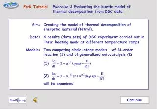
Continue. ForK Tutorial Exercise 3 Evaluating the kinetic model of thermal decomposition from DSC data. Aim: Creating the model of thermal decomposition of energetic material (tetryl).

E N D
Continue ForK TutorialExercise 3 Evaluating the kinetic model of thermal decomposition from DSC data Aim: Creating the model of thermal decomposition of energetic material (tetryl). Data: 4 results (data sets) of DSC experiment carried out in linear heating mode at different temperature ramps Models: Two competing single-stage models – of N-order reaction (1) and of generalized autocatalysis (2) (1) (2) will be examined Run Scoring
Select Estimation mode ForK Tutorial.Exercise 3 Evaluating kinetic model of thermal decomposition from DSC data
Viewing data on the Chart(using the “Show plot” command) View derivative responses (dQ/dt)
Click here to continue • Plan of evaluation procedure. • Getting rough estimates of kinetic parameters using data sets for temperature ramps 2 and 3 K/min for the competing models. • Validating the results by adding data sets for temperature ramps 0.5 and 1 K/min. • Selecting more appropriate model. • Running non-linear parameters estimation on the basis of 4 data sets.
0 0 2. Defining the model 1. Defining the 0 weight of data sets for 0.5 and 1 K/min (These data sets will me omitted when parameters estimation)
2. Estimating the initial guesson kinetic parameters (using the Arrhenius method)
Comparison of experiment and simulation based on initial parameters’ guess
Observation 1 Activation energy is too big for a reaction proceeding in the temperature interval 140220oC Next step is to check how the model predicts reaction course at smaller temperature ramps.
2. Viewing how the N-order model predicts reaction course 0 0 1. Returning to the weight=1 for data sets for 0.5 and 1 K/min
Observation 2 The N-order model doesn’t allow proper prediction of the reaction course – the simulated peaks appear later than experimental ones. Next step is to examine the alternative model of generalized autocatalysis. As earlier data sets for 2 and 3 K/min will be used for the analysis
0 0 2. Defining the model 1. Defining the 0 weight of data sets for 0.5 and 1 K/min
Estimating the initial guesson kinetic parameters (using the Arrhenius method)
Comparison of experiment and simulation based on initial parameters’ guess
Observation 1 Activation energy matches the reaction’s temperature interval though the shape of peaks simulated is somewhat distorted in comparison with the experimental peaks Next step is to check how the model predicts reaction course at lower temperature ramps.
2. Viewing how the autocatalytic model predicts reaction course 0 0 1. Returning to the weight=1 for data sets for 0.5 and 1 K/min
Observation 2 The autocatalytic model with the rough parameters estimates evaluated by using the simplified (Arrhenius) method doesn’t provide appropriate fit of peaks’ shape but predicts properly location of the peaks. Next step is to run non-linear parameters estimation and check whether the model is capable of fitting all the data available.
Adjusting numerical methods for parameters estimation and run estimation 3. Run nonlinear estimation 2. Defining numerical methods that will be used 1. Defining precision of numerical integration 0.0000001 0.0000001
Run optimization (using the tensor method in mode 1) Value of the objective function SS before estimation
Use the Plot for viewing the results on the Chart Resultant value of the objective function SS. Estimation has been stopped manually when no further progress had been observed
Comparison of experiment and simulation based on final parameters’ vector. Solid lines – simulation. 1. Integral responses.
Comparison of experiment and simulation based on final parameters’ vector. Solid lines – simulation. 2. Derivatives. The resultant kinetic model provides good fit of all the existing data. Estimates of the kinetic parameters are very reasonable. Conclusion: The kinetics created is in satisfactory agreement with experimental data and can be accepted for further use.
The last step is to save the kinetics evaluated into the data volume. Calling the Save as option
The 3rd Exercise is over. Press [Esc] to close presentation. If you have ForK installed we recommend to repeat this exercise by yourself using demo data