Spatio-temporal patterns in plant populations in small landscape elements
410 likes | 581 Views
Spatio-temporal patterns in plant populations in small landscape elements. Patrick Endels Laboratory for Forest, Nature and Landscape Research, KULeuven Vital Decosterstraat 102 B-3000 Leuven, Belgium Tel +32(0)16.32.97.69 Fax +32(0)16.32.97.60. outline. 1. research questions

Spatio-temporal patterns in plant populations in small landscape elements
E N D
Presentation Transcript
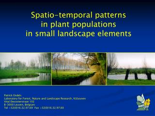
Spatio-temporal patterns in plant populations in small landscape elements Patrick Endels Laboratory for Forest, Nature and Landscape Research, KULeuven Vital Decosterstraat 102 B-3000 Leuven, Belgium Tel +32(0)16.32.97.69 Fax +32(0)16.32.97.60
outline 1. research questions 2. data recording 3. data management 4. analysis of temporal changes 5. analysis of spatial patterns 6. further analyses
general research questions • Impact of different ‘management’ regimes on demographic parameters of populations in small landscape elements? • barochory (Primula veris) vs. myrmecochory (Primula vulgaris) -> population dynamics & max. dispersal distance? • Impact of ‘management’ regimes on shape & tail of the dipsersal curve? • Relationship between dispersal distance & subsequent seedling/juvenile survival
data recording Primula vulgaris Primula veris
data recording • Primula vulgaris • 13 populations • forest edges (n=3) vs. • grazed parcel margins (n=4) vs. [1999-2002] • clearing of ditches & mowing (n=2) • restoration of mowing regime (n=1) [1999-2003] • changes in adjacent land use (n=1) [1999-2002]
data recording • Primula veris • 16 populations • graft (Voeren) (n=4) vs. • grazed parcel margins (n=4) vs. [2000-2002] • clearing of ditches & mowing (n=4) • restoration of calcareous grassland (n=2) [1999-2001] • (Voeren)
analysis of temporal changes Stage classification = a combination of both reproductive and size criteria Seedlings: individuals developed directly after the germination of seeds, with cotyledons still present and often also one ‘normal’ leaf-pair. Juveniles: immature plants without cotyledons and with only one rosette of leaves. Juveniles can only be distinguished from vegetative adults with one rosette by means of their size: an individual is considered as an adult when its leaf size is comparable to flowering plants in the same population; if leaf size is significantly smaller then the individual is assigned to the juvenile category. Vegetative adults: non-flowering individuals without cotyledons, with one or more rosettes, often showing signs of overwintering leaves. Leaf size is comparable to generative adults which are growing under similar conditions. Reproductive adults: plants baring one ore more flowering stalks, having one or more rosettes and often showing signs of older, overwintering leaves. These flowering adults were divided into three size categories according to the number of rosettes.
S J NFA RA1 RA2 RA3 analysis of temporal changes -> Moloney (1986) vs. empirical approach
YEAR t seedling juvenile NF Adult Repr Adult 1 (1 roz.) Repr Adult 2 (2-3 roz.) Repr Adult 3 (>3 roz.) seedling 0 0 0 F1 F2 F3 YEAR t+1 juvenile G21 L22 0 F4 F5 F6 NF Adult G31 G32 L33 L34 L35 L36 Repr Adult 1 G41 G42 G43 L44 L45 L46 Repr Adult 2 G51 G52 G53 G54 L55 L56 Repr Adult 3 0 0 G63 G64 G62 L66 analysis of temporal changes n(t + 1) = A n(t)
sensitivity analysis Triangular plot of composite elasticity values for growth (G), statis (L) and fecundity (F) species populations (Silvertown et al. 1992, 1996)
sites [P. vulgaris] grazed parcel margins forest edges ditch clearing (+mowing)
population growth rates [P. vulgaris] tests of within-subjects contrasts F P YEAR 11.019 < 0.05 YEAR * MANAGEMENT 6.533 < 0.05 tests of between-subjects effects F P MANAGEMENT 6.5650 < 0.05 repeated measures ANOVA:
sensitivity analysis [P. vulgaris] forest edge grazed mown/cleared
population growth rates [P. vulgaris] ? different mowing regimes
sensitivity analysis [P. vulgaris] not mown mown 1mown 2
population growth rates [P. vulgaris] clearing (+mowing) of ditches
population growth rates [P. vulgaris] ! changes in adjacent land use
sensitivity analysis [P. vulgaris] arable field grassland
sites [P. veris] clearing / mowing graft (Voeren) grassland margins
population growth rates [P. veris] repeated measures ANOVA:
sensitivity analysis [P. veris] L G L F F
conclusions temporal analysis [P. vulgaris] - 2 (a) mowing regime - first year : effect of mowing once or twice a year ≅ - In the “long run”: only mowing twice a year (July & October) efficient to counter population senescence to lift λ above 1 (b) ditch clearing regime (& mowing of ditch bank) - large impact on population growth rate (depending on intensity) - temporarily higher mortality levels - compensated by higher seedling recruitment and survival c)changes in adjacent land use - grassland -> arable field: (1) effect on population growth rate and (2) populations more responsive to survival of veg. adults - population quickly recovers when the original land use is restored
conclusions temporal analysis [P. vulgaris & P. veris] - 3 in general: - disturbances of any kind force populations into earlier stages of the successional G-L-F trajectory (Silvertown et al. 1996) - however, these more dynamic populations (i.e. more dependent on / responsive to fecundity and growth) are not necessarily associated with higher population growth rates (’s)
analysis of spatial patterns calculation of dispersal distances dispersal curves for the two species for different management regimes -> tail (max. dispersal distance)?! dispersal distance and survival -> Janzen (1970)-Connell (1971) vs. Hubbell (1979)
dispersal distance & management regime [P. vulgaris] max. = 2.45 m max. = 1.04 m max. = 2.62 m mean = 0.26 m mean = 0.29 m mean = 0.42 m ab b a max. = 0.61 m max. = 3.89 m max. = 2.12 m mean = 0.25 m mean = 0.38 m mean = 0.17 m b b a max. = 0.54 m max. = 1.26 m max. = 1.89 m mean = 0.16 m mean = 0.19 m mean = 0.36 m a b c
dispersal distance & management regime [P. veris] max. = 0.57 m max. = 5.49 m mean = 0.10 m mean = 0.23 m < P < 0.001 max. = 0.47 m max. = 2.60 m mean = 0.15 m mean = 0.25 m ≈ ? n.s
dispersal distance & survival P. vulgaris Wald χ² = 44.285 n = 1720 P < 0.001
dispersal distance & survival P. vulgaris Wald χ² = 4.425 n = 91;P = 0.035 Wald χ² = 0.065 n = 271; P = 0.798 Wald χ² = 53.200 n = 1344; P < 0.001 dispersal distance
dispersal distance & survival P. veris Wald χ² = 15.223 n = 2815 P < 0.001
dispersal distance & survival P. veris Wald χ² = 7.141 n = 344;P = 0.008 Wald χ² = 16.137 n = 2438; P < 0.001 dispersal distance
spatial patterns: conclusions J.-C. J.-C. J.-C. H.
further analyses (1) temporal changes - relationship with reproductive output - comparison of population growth rate by randomization tests - LTRE (mowing regime P. vulgaris, management regime P. veris) - stochastic population modelling (Caswell 2001, Tuljapulkar & Caswell 1997)
further analyses (2) spatial patterns - relationship between aggregation & dispersal distance (calculation of Ripley’s K & comparison between management regimes) - aggregation and flower morph types ? - ? ? ? incorporating plant performance -link with recruitment / population dynamics ?