Download
1 / 23
240 likes | 403 Views
Lecture 13. ANNOUNCEMENTS Midterm #1 (Thursday 10/11, 3:30PM-5:00PM) location: 106 Stanley Hall: Students with last names starting with A-L 306 Soda Hall: Students with last names starting with M-Z EECS Dept. policy re: academic dishonesty will be strictly followed ! HW#7 is posted online.

E N D
Lecture 13 ANNOUNCEMENTS • Midterm #1 (Thursday 10/11, 3:30PM-5:00PM) location: • 106 Stanley Hall: Students with last names starting with A-L • 306 Soda Hall: Students with last names starting with M-Z • EECS Dept. policy re: academic dishonesty will be strictly followed! • HW#7 is posted online. OUTLINE • Cascode Stage: final comments • Frequency Response • General considerations • High-frequency BJT model • Miller’s Theorem • Frequency response of CE stage Reading: Chapter 11.1-11.3
Cascoding Cascode? • Recall that the output impedance seen looking into the collector of a BJT can be boosted by as much as a factor of b, by using a BJT for emitter degeneration. • If an extra BJT is used in the cascode configuration, the maximum output impedance remains bro1.
Cascode Amplifier • Recall that voltage gain of a cascode amplifier is high, because Rout is high. • If the input is applied to the base of Q2 rather than the base of Q1, however, the voltage gain is not as high. • The resulting circuit is a CE amplifier with emitter degeneration, which has lower Gm.
Review: Sinusoidal Analysis • Any voltage or current in a linear circuit with a sinusoidal source is a sinusoid of the same frequency (w). • We only need to keep track of the amplitude and phase, when determining the response of a linear circuit to a sinusoidal source. • Any time-varying signal can be expressed as a sum of sinusoids of various frequencies (and phases). Applying the principle of superposition: • The current or voltage response in a linear circuit due to a time-varying input signal can be calculated as the sum of the sinusoidal responses for each sinusoidal component of the input signal.
High Frequency “Roll-Off” in Av • Typically, an amplifier is designed to work over a limited range of frequencies. • At “high” frequencies, the gain of an amplifier decreases.
Av Roll-Off due to CL • A capacitive load (CL) causes the gain to decrease at high frequencies. • The impedance of CL decreases at high frequencies, so that it shunts some of the output current to ground.
Frequency Response of the CE Stage • At low frequency, the capacitor is effectively an open circuit, and Avvs.w is flat. At high frequencies, the impedance of the capacitor decreases and hence the gain decreases. The “breakpoint” frequency is 1/(RCCL).
Amplifier Figure of Merit (FOM) • The gain-bandwidth product is commonly used to benchmark amplifiers. • We wish to maximize both the gain and the bandwidth. • Power consumption is also an important attribute. • We wish to minimize the power consumption. • Operation at low T, low VCC, and with small CL superior FOM
Bode Plot • The transfer function of a circuit can be written in the general form • Rules for generating a Bode magnitude vs. frequency plot: • As w passes each zero frequency, the slope of |H(jw)| increases by 20dB/dec. • As w passes each pole frequency, the slope of |H(jw)| decreases by 20dB/dec. A0 is the low-frequency gain wzjare “zero” frequencies wpj are “pole” frequencies
Bode Plot Example • This circuit has only one pole at ωp1=1/(RCCL); the slope of |Av|decreases from 0 to -20dB/dec at ωp1. • In general, if node j in the signal path has a small-signal resistance of Rjto ground and a capacitance Cj to ground, then it contributes a pole at frequency (RjCj)-1
High-Frequency BJT Model • The BJT inherently has junction capacitances which affect its performance at high frequencies. Collector junction: depletion capacitance, Cm Emitter junction: depletion capacitance, Cje, and also diffusion capacitance, Cb.
BJT High-Frequency Model (cont’d) • In an integrated circuit, the BJTs are fabricated in the surface region of a Si wafer substrate; another junction exists between the collector and substrate, resulting in substrate junction capacitance, CCS. BJT cross-section BJT small-signal model
Example: BJT Capacitances • The various junction capacitances within each BJT are explicitly shown in the circuit diagram on the right.
Transit Frequency, fT • The “transit” or “cut-off” frequency, fT, is a measure of the intrinsic speed of a transistor, and is defined as the frequency where the current gain falls to 1. Conceptual set-up to measure fT
Dealing with a Floating Capacitance • Recall that a pole is computed by finding the resistance and capacitance between a node and GROUND. • It is not straightforward to compute the pole due to Cm1 in the circuit below, because neither of its terminals is grounded.
Miller’s Theorem • If Av is the voltage gain from node 1 to 2, then a floating impedance ZF can be converted to two grounded impedances Z1 and Z2:
Miller Multiplication • Applying Miller’s theorem, we can convert a floating capacitance between the input and output nodes of an amplifier into two grounded capacitances. • The capacitance at the input node is larger than the original floating capacitance.
… Applying Miller’s Theorem Note that wp,out > wp,in
Direct Analysis of CE Stage • Direct analysis yields slightly different pole locations and an extra zero: