Download
1 / 47
470 likes | 571 Views
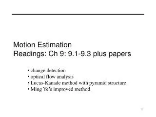
Motion Estimation Readings: Ch 9: 9.1-9.3 plus papers. change detection optical flow analysis Lucas-Kanade method with pyramid structure Ming Ye’s improved method. Why estimate motion?. We live in a 4-D world Wide applications Object Tracking Camera Stabilization Image Mosaics

E N D
Motion EstimationReadings: Ch 9: 9.1-9.3 plus papers • change detection • optical flow analysis • Lucas-Kanade method with pyramid structure • Ming Ye’s improved method
Why estimate motion? • We live in a 4-D world • Wide applications • Object Tracking • Camera Stabilization • Image Mosaics • 3D Shape Reconstruction (SFM) • Special Effects (Match Move)
Change detection for surveillance • Video frames: F1, F2, F3, … • Objects appear, move, disappear • Background pixels remain the same (simple case) • How do you detect the moving objects? • Simple answer: pixelwise subtraction
Example: Person detected entering room • Pixel changes detected as difference components • Regions are (1) person, (2) opened door, and (3) computer monitor. • System can know about the door and monitor. Only the person region is “unexpected”.
Change Detection via Image Subtraction for each pixel [r,c] if (|I1[r,c] - I2[r,c]| > threshold) then Iout[r,c] = 1 else Iout[r,c] = 0 Perform connected components on Iout. Remove small regions. Perform a closing with a small disk for merging close neighbors. Compute and return the bounding boxes B of each remaining region. What assumption does this make about the changes?
Change analysis Known regions are ignored and system attends to the unexpected region of change. Region has bounding box similar to that of a person. System might then zoom in on “head” area and attempt face recognition.
Key assumptions • color constancy: a point in H looks the same in I • For grayscale images, this is brightness constancy • small motion: points do not move very far • This is called the optical flow problem Problem definition: optical flow • How to estimate pixel motion from image H to image I? • Solve pixel correspondence problem • given a pixel in H, look for nearby pixels of the same color in I
Optical flow constraints (grayscale images) • Let’s look at these constraints more closely • brightness constancy: Q: what’s the equation? H(x, y) = I(x+u, y+v) • small motion: (u and v are less than 1 pixel) • suppose we take the Taylor series expansion of I:
Optical flow equation • Combining these two equations The x-component of the gradient vector. What is It ? The time derivative of the image at (x,y) How do we calculate it?
Optical flow equation • Q: how many unknowns and equations per pixel? 1 equation, but 2 unknowns (u and v) • Intuitively, what does this constraint mean? • The component of the flow in the gradient direction is determined • The component of the flow parallel to an edge is unknown
Lukas-Kanade flow • How to get more equations for a pixel? • Basic idea: impose additional constraints • most common is to assume that the flow field is smooth locally • one method: pretend the pixel’s neighbors have the same (u,v) • If we use a 5x5 window, that gives us 25 equations per pixel!
RGB version • How to get more equations for a pixel? • Basic idea: impose additional constraints • most common is to assume that the flow field is smooth locally • one method: pretend the pixel’s neighbors have the same (u,v) • If we use a 5x5 window, that gives us 25*3 equations per pixel!
Solution: solve least squares problem • minimum least squares solution given by solution (in d) of: • The summations are over all pixels in the K x K window • This technique was first proposed by Lukas & Kanade • for stereo matching (1981) Lukas-Kanade flow • Prob: we have more equations than unknowns
Conditions for solvability • Optimal (u, v) satisfies Lucas-Kanade equation • When is This Solvable? • ATA should be invertible • ATA should not be too small due to noise • eigenvalues l1 and l2 of ATA should not be too small • ATA should be well-conditioned • l1/ l2 should not be too large (l1 = larger eigenvalue)
Edges cause problems • large gradients, all the same • large l1, small l2
Low texture regions don’t work • gradients have small magnitude • small l1, small l2
High textured region work best • gradients are different, large magnitudes • large l1, large l2
Errors in Lukas-Kanade • What are the potential causes of errors in this procedure? • Suppose ATA is easily invertible • Suppose there is not much noise in the image • When our assumptions are violated • Brightness constancy is not satisfied • The motion is not small • A point does not move like its neighbors • window size is too large • what is the ideal window size?
Revisiting the small motion assumption • Is this motion small enough? • Probably not—it’s much larger than one pixel (2nd order terms dominate) • How might we solve this problem?
u=1.25 pixels u=2.5 pixels u=5 pixels u=10 pixels image H image I image H image I Gaussian pyramid of image H Gaussian pyramid of image I Coarse-to-fine optical flow estimation
warp & upsample run iterative L-K . . . image J image I image H image I Gaussian pyramid of image H Gaussian pyramid of image I Coarse-to-fine optical flow estimation run iterative L-K
A Few Details • Top Level • Apply L-K to get a flow field representing the flow from the first frame to the second frame. • Apply this flow field to warp the first frame toward the second frame. • Rerun L-K on the new warped image to get a flow field from it to the second frame. • Repeat till convergence. • Next Level • Upsample the flow field to the next level as the first guess of the flow at that level. • Apply this flow field to warp the first frame toward the second frame. • Rerun L-K and warping till convergence as above. • Etc.
The Flower Garden Video What should the optical flow be?
Robust Visual Motion Analysis: Piecewise-Smooth Optical Flow Ming Ye Electrical Engineering University of Washington
Structure From Motion Rigid scene + camera translation Estimated horizontal motion Depth map
Scene Dynamics Understanding • Surveillance • Event analysis • Video compression Brighter pixels => larger speeds. Estimated horizontal motion Motion boundaries are smooth. Motion smoothness
Tracking results Target Detection and Tracking A tiny airplane --- only observable by its distinct motion
Estimating Piecewise-Smooth Optical Flow with Global Matching and Graduated Optimization Problem Statement: Assuming only brightness conservation and piecewise-smooth motion, find the optical flow to best describe the intensity change in three frames.
Approach: Matching-Based Global Optimization • Step 1. Robust local gradient-based method for • high-quality initial flow estimate. • Step 2. Global gradient-based method to improve the • flow-field coherence. • Step 3. Global matching that minimizes energy by a • greedy approach.
Global Energy Design • Global energy • V is the optical flow field. • Vs is the optical flow at pixel (site) s. • EB is the brightness conservation error. • ES is the flow smoothness error in a neighborhood about pixel s.
Global Energy Design • Brightness error • warping error I-(Vs) is the warped intensity in the previous frame. I+(Vs) is the warped intensity in the next frame. I- I I+ Error function: where is a scale parameter.
Global Energy Design • Smoothness error Smoothness error is computed in a neighborhood around pixel s. Vnw Vn Vne Vw Vs Ve Vsw Vs Vse Error function:
Level p warp Calculate gradients Local OFC Global OFC Global matching Level p-1 Projection Image pyramid Overall Algorithm
Advantages • Best of Everything • Local OFC • High-quality initial flow estimates • Robust local scale estimates • Global OFC • Improve flow smoothness • Global Matching • The optimal formulation • Correct errors caused by poor gradient quality and hierarchical process • Results: fast convergence, high accuracy, simultaneous motion boundary detection
Experiments • Experiments were run on several standard test videos. • Estimates of optical flow were made for the middle • frame of every three. • The results were compared with the Black and • Anandan algorithm.
TS: Translating Squares • Homebrew, ideal setting, test performance upper bound 64x64, 1pixel/frame Groundtruth (cropped), Our estimate looks the same
TS: Flow Estimate Plots LS BA S1 (S2 is close) S3 looks the same as the groundtruth. • S1, S2, S3: results from our Step I, II, III (final)
BA 2.60 0.128 0.0724 S3 0.248 0.0167 0.00984 TT: Translating Tree 150x150 (Barron 94) BA S3 e: error in pixels, cdf: culmulative distribution function for all pixels
BA 6.36 0.182 0.114 S3 2.60 0.0813 0.0507 DT: Diverging Tree 150x150 (Barron 94) BA S3
BA 2.71 0.185 0.118 S3 1.92 0.120 0.0776 YOS: Yosemite Fly-Through 316x252 (Barron, cloud excluded) BA S3
TAXI: Hamburg Taxi 256x190, (Barron 94) max speed 3.0 pix/frame LMS BA Ours Error map Smoothness error
Traffic 512x512 (Nagel) max speed: 6.0 pix/frame BA Ours Error map Smoothness error
Pepsi Can 201x201 (Black) Max speed: 2pix/frame Ours Smoothness error BA
FG: Flower Garden 360x240 (Black) Max speed: 7pix/frame BA LMS Ours Error map Smoothness error