Download
1 / 99
1k likes | 1.02k Views
This article covers the basics of motion planning in autonomous robots and digital actors. It discusses the discretization of state spaces, various discretization techniques, intruder finding problems, information states, criticality-based discretization, and challenges with articulated robot motion planning. It also explores configuration spaces, obstacle mapping, grid-based vs. criticality-based discretization, and probabilistic roadmap methods for efficient motion planning.

E N D
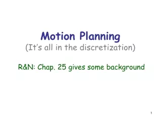
Motion Planning(It’s all in the discretization)R&N: Chap. 25 gives some background
Motion planning is the ability for an agent to compute its own motions in order to achieve certain goals. All autonomous robots and digital actors should eventually have this ability
Basic problem • Point robot in a 2-dimensional workspace with obstacles of known shape and position • Find a collision-free path between a start and a goal position of the robot
Basic problem • Each robot position (x,y) can be seen as a state • Continuous state space • Then each state has an infinity of successors • We need to discretize the state space (x,y)
Two Possible Discretizations Grid-based Criticality-based
Two Possible Discretizations Grid-based Criticality-based But this problem is very simple How do these discretizations scale up?
cleared region 2 4 5 6 Intruder Finding Problem robot robot’s visibilityregion • A moving intruder is hiding in a 2-D workspace • The robot must “sweep” the workspace to find the intruder • Both the robot and the intruder are points hiding region 1 3
Easy to test: “Hole” in the workspace Does a solution always exist? No ! Hard to test: No “hole” in the workspace
a = 0 or 1 c = 0 or 1 b = 0 or 1 (x,y) 0 cleared region 1 hidding region Information State • Example of an information state = (x,y,a=1,b=1,c=0) • An initial state is of the form (x,y,1, 1, ..., 1) • A goal state is any state of the form (x,y,0,0, ..., 0)
b=1 b=0 a=0 a=0 b=1 a=0 Information state is unchanged Critical line Critical Line
A E B C D Criticality-Based Discretization Each of the regions A, B, C, D, and E consists of “equivalent” positions of the robot, so it’s sufficient to consider a single position per region
A (C, 1, 1) (B, 1) (D, 1) E B C D Criticality-Based Discretization
A (C, 1, 1) (B, 1) (D, 1) E B C D (C, 1, 0) (E, 1) Criticality-Based Discretization
A (C, 1, 1) (B, 1) (D, 1) E B C D (C, 1, 0) (E, 1) (B, 0) (D, 1) Criticality-Based Discretization
A (C, 1, 1) (B, 1) (D, 1) E C D (C, 1, 0) (E, 1) (B, 0) (D, 1) Criticality-Based Discretization B Much smaller search tree than with grid-based discretization !
Grid-Based Discretization • Ignores critical lines Visits many “equivalent” states • Many information states per grid point • Potentially very inefficient
But ... Criticality-based discretization does not scale well in practice when the dimensionality of the continuous space increases (It becomes prohibitively complex to define and compute)
Motion Planning for an Articulated Robot Find a path to a goal configuration that satisfies various constraints: collision avoidance, equilibrium, etc...
Configuration Space of an Articulated Robot • A configuration of a robot is a list of non-redundant parameters that fully specify the position and orientation of each of its bodies • In this robot, one possible choice is: (q1, q2) The configuration space(C-space) has 2 dimensions
How many dimensions has the C-space of these 3 rings? Answer: 35 = 15
q q q q q 1 3 0 n 4 Every robot maps to a point in its configuration space ... ~40 D 15 D 6 D 12 D ~65-120 D
q q q q q 1 3 0 n 4 ... and every robot path is a curve in configuration space
q q q q q 1 3 0 n 4 But how do obstacles (and other constraints) map in configuration space? ~40 D 15 D 6 D 12 D ~65-120 D
C-space “reduces” motion planning to finding a path for a point But how do the obstacle constraints map into C-space ?
A Simple Example: Two-Joint Planar Robot Arm • Problems: • Geometric complexity • Space dimensionality
Continuous state space Discretization C-space Search
About Discretization • Dimensionality + geometric complexity Criticality-based discretization turns out to be prohibitively complex • Dimensionality Grid-based discretization leads to impractically large state spaces for dim(C-space) 6 Each grid node has 3n-1 neighbors, where n = dim(C-space)
Robots with many joints: Modular Self-Reconfigurable Robots Millipede-like robot with 13,000 joints (M. Yim) (S. Redon)
forbidden space feasible space Probabilistic Roadmap (PRM) n-dimensionalC-space
Probabilistic Roadmap (PRM) Configurations are sampled by picking coordinates at random
Probabilistic Roadmap (PRM) Configurations are sampled by picking coordinates at random
Probabilistic Roadmap (PRM) Sampled configurations are tested for collision (feasibility)
Probabilistic Roadmap (PRM) The collision-free configurations are retained as “milestones” (states)
Probabilistic Roadmap (PRM) Each milestone is linked by straight paths to its k-nearest neighbors
Probabilistic Roadmap (PRM) Each milestone is linked by straight paths to its k-nearest neighbors
Probabilistic Roadmap (PRM) The collision-free links are retained to form the PRM (state graph)
g s Probabilistic Roadmap (PRM) The start and goal configurations are connected to nodes of the PRM
g s Probabilistic Roadmap (PRM) The PRM is searched for a path from s to g
Continuous state space Discretization Search A*
Why Does PRM Work? Because most feasible spaces verifies some good geometric (visibility) properties
Why Does PRM Work? In most feasible spaces, every configuration “sees” a significant fraction of the feasible space A relatively small number of milestones and connections between them are sufficient to cover most feasible spaces with high probability
S1 S2 Lookout of S1 Narrow-Passage Issue The lookout of a subset S of the feasible space is the set of all configurations in S from which it is possible to “see” a significant fraction of the feasible space outside S The feasible space isexpansiveif all of its subsets have a large lookout
Probabilistic Completeness of a PRM Motion Planner In an expansive feasible space, the probability that a PRM planner with uniform sampling strategy finds a solution path, if one exists, goes to 1 exponentially with the number of milestones (~ running time) A PRM planner can’t detect that no path exists. Like A*, it must be allocated a time limit beyond which it returns that no path exists. But this answer may be incorrect. Perhaps the planner needed more time to find one !
Continuous state space Discretization C-space Search
Sampling Strategies • Issue: Where to sample configurations? That is, which probabilistic distribution to use? • Example: Two-stage sampling strategy: • Construct initial PRM with uniform sampling • Identify milestones that have few connections to their close neighbors • Sample more configurations around them Greater density of milestones in “difficult” regions of the feasible space