Download
1 / 23
230 likes | 526 Views
L21: “Irregular” Graph Algorithms. November 11, 2010. Administrative. Class cancelled, November 16! Guest Lecture, November 18, Matt Might CUDA Projects status Available on CADE Linux machines (lab1 and lab3) and Windows machines (lab5 and lab6)

E N D
L21: “Irregular” Graph Algorithms November 11, 2010
Administrative • Class cancelled, November 16! • Guest Lecture, November 18, Matt Might • CUDA Projects status • Available on CADE Linux machines (lab1 and lab3) and Windows machines (lab5 and lab6) • libcutil.a (in SDK) only installed on Linux machines • Windows instructions, but cannot do timings
Programming Assignment #3: Simple CUDADue Monday, November 22, 11:59 PM Today we will cover Successive Over Relaxation. Here is the sequential code for the core computation, which we parallelize using CUDA: for(i=1;i<N-1;i++) { for(j=1;j<N-1;j++) { B[i][j] = (A[i-1][j]+A[i+1][j]+A[i][j-1]+A[i][j+1])/4; } } You are provided with a CUDA template (sor.cu) that (1) provides the sequential implementation; (2) times the computation; and (3) verifies that its output matches the sequential code.
Programming Assignment #3, cont. • Your mission: • Write parallel CUDA code, including data allocation and copying to/from CPU • Measure speedup and report • 45 points for correct implementation • 5 points for performance • Extra credit (10 points): use shared memory and compare performance
Programming Assignment #3, cont. • You can install CUDA on your own computer • http://www.nvidia.com/cudazone/ • How to compile under Linux and MacOS • Visual Studio (no cutil library for validation) • http://www.cs.utah.edu/~mhall/cs4961f10/CUDA-VS08.pdf • Version 3.1 in CADE labs lab1 and lab3: See Makefile at http://www.cs.utah.edu/~mhall/cs4961f10/Makefile • Turn in • Handin cs4961 proj3 <file> (includes source file and explanation of results)
Outline • Irregular parallel computation • Sparse matrix operations (last time) and graph algorithms (this time) • Dense graph algorithms (shortest path) • Sparse graph algorithms (shortest path and maximal independent set) • Sources for this lecture: • Kathy Yelick/Jim Demmel (UC Berkeley): CS 267, Spr 07 • http://www.eecs.berkeley.edu/~yelick/cs267_sp07/lectures • “Implementing Sparse Matrix-Vector Multiplication on Throughput Oriented Processors,” Bell and Garland (Nvidia), SC09, Nov. 2009. • Slides accompanying textbook “Introduction to Parallel Computing” by Grama, Gupta, Karypis and Kumar • http://www-users.cs.umn.edu/~karypis/parbook/
Representing Graphs An undirected graph and its adjacency matrix representation. An undirected graph and its adjacency list representation.
Common Challenges in Graph Algorithms All of these issues must be addressed by a graph partitioning algorithm that maps individual subgraphs to individual processors. • Localizing portions of the computation • How to partition the workload so that nearby nodes in the graph are mapped to the same processor? • How to partition the workload so that edges that represent significant communication are co-located on the same processor? • Balancing the load • How to give each processor a comparable amount of work? • How much knowledge of the graph do we need to do this since complete traversal may not be realistic?
Start with Dense Graphs • Partitioning problem is straightforward for dense graphs • We’ll use an adjacency matrix and partition the matrix just like we would a data-parallel matrix computation • Examples • Single-source shortest path and all-pairs shortest path
Single-Source shortest path (parallel) • Each processor is assigned a portion of V, l and w • Which part? • Involves a global reduction to pick minimum
All Pairs Shortest Path • Given a weighted graph G(V,E,w), the all-pairs shortest paths problem is to find the shortest paths between all pairs of vertices vi, vj ∈ V. • We discuss two versions • Extend single-source shortest path • Matrix-multiply based solution (sparse or dense graph)
All-Pairs Parallel based on Dijkstra’s Algorithm • Source partitioned: • Execute each of the n single-source shortest path problems on a different processor • That is, using n processors, each processor Pi finds the shortest paths from vertex vi to all other vertices by executing Dijkstra's sequential single-source shortest paths algorithm. • Pros and Cons? Data structures? • Source parallel: • Use a parallel formulation of the shortest path problem to increase concurrency. • Each of the shortest path problems is further executed in parallel. We can therefore use up to n2 processors. • Given p processors (p > n), each single source shortest path problem is executed by p/n processors.
All-Pairs Shortest Paths:Matrix-Multiplication Based Algorithm The product of weighted adjacency matrix with itself returns a matrix that contains shortest paths of length 2 between any pair of nodes. It follows from this argument that An contains all shortest paths.
Sparse Shortest Path (using adjacency list) w(u,v) is a field of the element in v’s adjacency list representing u
Parallelizing Johnson’s Algorithm Selecting vertices from the priority queue is the bottleneck We can improve this by using multiple queues, one for each processor. Each processor builds its priority queue only using its own vertices. When process Pi extracts the vertex u ∈ Vi, it sends a message to processes that store vertices adjacent to u. Process Pj, upon receiving this message, sets the value of l[v] stored in its priority queue to min{l[v],l[u] + w(u,v)}.
Maximal Independent Set (used in Graph Coloring) A set of vertices I ⊂ V is called independent if no pair of vertices in I is connected via an edge in G. An independent set is called maximal if by including any other vertex not in I, the independence property is violated.
Sequential MIS algorithm Simple algorithms start by MIS I to be empty, and assigning all vertices to a candidate set C. Vertex v from C is moved into I and all vertices adjacent to v are removed from C. This process is repeated until C is empty. This process is inherently serial!
Foundation for Parallel MIS algorithm Parallel MIS algorithms use randomization to gain concurrency (Luby's algorithm for graph coloring). Initially, each node is in the candidate set C. Each node generates a (unique) random number and communicates it to its neighbors. If a node’s number exceeds that of all its neighbors, it joins set I. All of its neighbors are removed from C. This process continues until C is empty. On average, this algorithm converges after O(log|V|) such steps.
Parallel MIS Algorithm (Shared Memory) We use three arrays, each of length n - I, which stores nodes in MIS, C, which stores the candidate set, and R, the random numbers. Partition C across p processors. Each processor generates the corresponding values in the R array, and from this, computes which candidate vertices can enter MIS. The C array is updated by deleting all the neighbors of vertices that entered MIS. The performance of this algorithm is dependent on the structure of the graph.
Definition of Graph Partitioning • Given a graph G = (N, E, WN, WE) • N = nodes (or vertices), • WN = node weights • E = edges • WE = edge weights • Ex: N = {tasks}, WN = {task costs}, edge (j,k) in E means task j sends WE(j,k) words to task k • Choose a partition N = N1 U N2 U … U NP such that • The sum of the node weights in each Nj is “about the same” • The sum of all edge weights of edges connecting all different pairs Nj and Nk is minimized • Ex: balance the work load, while minimizing communication • Special case of N = N1 U N2: Graph Bisection 2 (2) 1 3 (1) 4 1 (2) 2 4 (3) 3 1 2 2 5 (1) 8 (1) 1 6 5 6 (2) 7 (3)
Definition of Graph Partitioning • Given a graph G = (N, E, WN, WE) • N = nodes (or vertices), • WN = node weights • E = edges • WE = edge weights • Ex: N = {tasks}, WN = {task costs}, edge (j,k) in E means task j sends WE(j,k) words to task k • Choose a partition N = N1 U N2 U … U NP such that • The sum of the node weights in each Nj is “about the same” • The sum of all edge weights of edges connecting all different pairs Nj and Nk is minimized (shown in black) • Ex: balance the work load, while minimizing communication • Special case of N = N1 U N2: Graph Bisection 2 (2) 1 3 (1) 4 1 (2) 2 4 (3) 3 1 2 2 5 (1) 8 (1) 1 6 5 6 (2) 7 (3)
Summary of Lecture • Summary • Regular computations are easier to schedule, more amenable to data parallel programming models, easier to program, etc. • Performance of irregular computations is heavily dependent on representation of data • Choosing this representation may depend on knowledge of the problem, which may only be available at run time • Next Time • Introduction to parallel graph algorithms • Minimizing bottlenecks