Download

1 / 21
210 likes | 337 Views
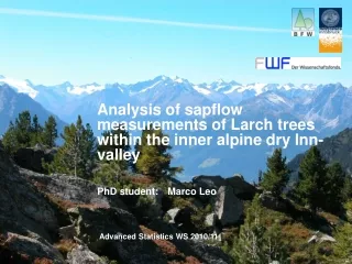
Analysis of sapflow measurements of Larch trees within the inner alpine dry Inn-valley. PhD student: Marco Leo. Advanced Statistics WS 2010/11. Overview. Background Principle of sapflow measurements Collection of environmental data Statistical analysis of time series data

E N D
Analysis of sapflow measurements of Larch trees within the inner alpine dry Inn-valley PhD student: Marco Leo Advanced Statistics WS 2010/11
Overview • Background • Principleofsapflowmeasurements • Collectionof environmental data • Statistical analysisof time seriesdata • Descriptivestatistics • Multiple linear regression • Autocorrelation
Principle of sapflow measurements • Two sensors installed into the sapwood • The top sensor is heated • Temperature difference between the sensors • Calculation of the sapflow density [ml cm2 min] • Relative sapflow for data interpretation ! • Dependent variable
Dependence of environmental parameters • Collected environmental data: (independent variables)
What is Autocorrelation ? Autocorrelation is the correlation of a signal with itself (Parr 1999). part of the data:
Testing Autocorrelation Durbin Watson Test H0 : α = 0 → No Autocorrelation H1 : α ≠ 0 → Autocorrelation durbinWatsonTest(model_LA_2) lag Autocorrelation D-W Statistic p-value 1 0.5097381 0.9703643 0 Alternative hypothesis: rho != 0
Determine the strength of the Autocorrelation • Autocorrelation Function (ACF) • Partial Autocorrelation Function (PACF) Yt = α Yt-1 + εt
Time series model - ARIMA • Elimination of the Autocorrelation • Results: • Summary • Table with coefficients and standard errors
Multicollinearity • Variance Inflation Factors (vif) • tolerance = 1/vif
Differential effect of the independent variables bj…regression coefficient Sxj…standard deviation of xj Sy…standard deviation of y
Helpful R commands/featuresforusing time seriesdata: • Arima model: the output differs from a lm model • Residual diagnostic • plot(model_LA_2$resid,xlab="day of year",main="VPD2 model“) • Create lines to get an overview of diagnostic plots • abline(h=0,col="red") • abline(0,1,col="red")